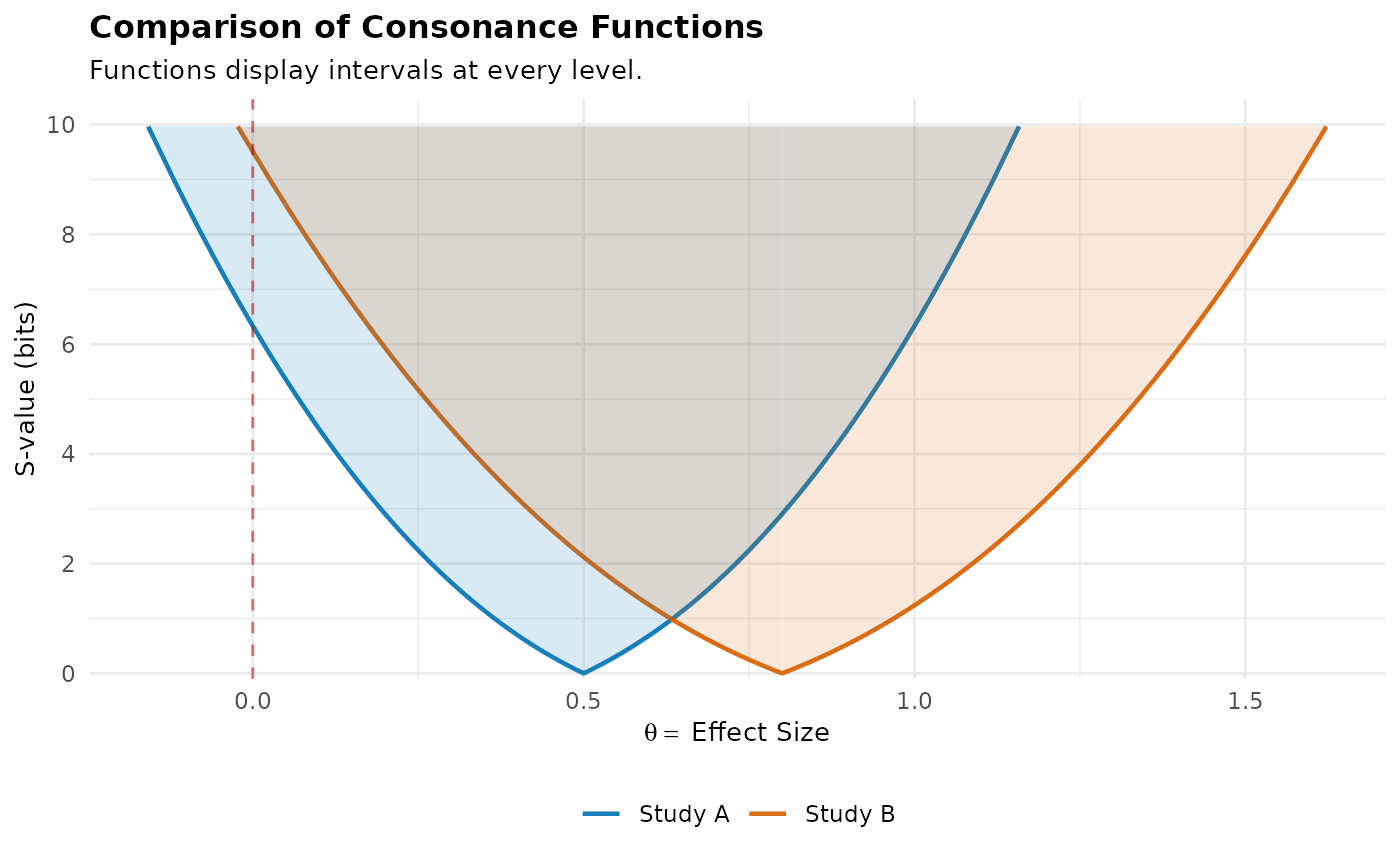
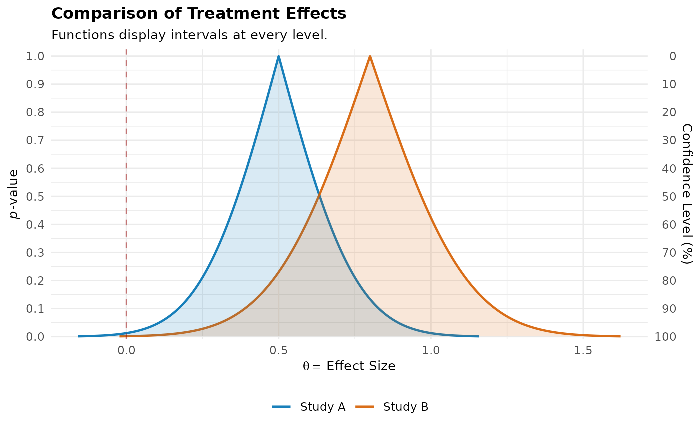
Overlays multiple consonance or surprisal functions on a single plot for direct visual comparison of effect estimates across groups, time periods, or studies.
plot_multi(..., type = "c", measure = "default", nullvalue = NULL,
  position = "pyramid", title = "Comparison of Consonance Functions",
  subtitle = "Functions display intervals at every level.",
  xaxis = expression(theta == ~"Effect Size"),
  yaxis1 = expression(paste(italic(p), "-value")),
  yaxis2 = "Confidence Level (%)", colors = NULL, alpha = 0.15,
  legend.position = "bottom")
Arguments
- ...
Named concurve dataframes to compare. Names become legend labels. Alternatively, pass a single named list of dataframes.
- type
Character. Type of function to plot: "c" for consonance (default), "s" for surprisal.
- measure
Character. Scale type: "default" for linear, "ratio" for log scale (odds ratios, hazard ratios, etc.).
- nullvalue
Numeric. Value(s) to mark with vertical reference line(s). Use single value (e.g., 0) or vector for range (e.g., c(-0.5, 0.5)).
- position
Character. Orientation of consonance function: "pyramid" (default) or "inverted".
- title
Character. Plot title.
- subtitle
Character. Plot subtitle.
- xaxis
Character or expression. X-axis label.
- yaxis1
Character or expression. Primary y-axis label.
- yaxis2
Character. Secondary y-axis label (for CI levels).
- colors
Character vector. Colors for each curve. If NULL, uses colorblind-friendly palette.
- alpha
Numeric. Transparency for ribbon fill (0-1). Default is 0.15.
- legend.position
Character or numeric vector. Legend position. Default is "bottom".
Value
A ggplot2 object (inheriting from ggplot).
Details
Curve names (passed as named arguments) are automatically used as legend labels.
For example, plot_multi("Study A" = curve1, "Study B" = curve2) will use
"Study A" and "Study B" as labels in the legend.
See also
Examples
# Overlay estimates from two studies. Names become legend labels.
study_a <- curve_from_se(estimate = 0.5, se = 0.20)
study_b <- curve_from_se(estimate = 0.8, se = 0.25)
plot_multi(
"Study A" = study_a[[1]],
"Study B" = study_b[[1]],
nullvalue = 0,
title = "Comparison of Treatment Effects"
)
 # A named list works too. The surprisal scale is often easier to read
# when the curves overlap heavily.
plot_multi(
list("Study A" = study_a[[1]], "Study B" = study_b[[1]]),
type = "s",
nullvalue = 0
)
# A named list works too. The surprisal scale is often easier to read
# when the curves overlap heavily.
plot_multi(
list("Study A" = study_a[[1]], "Study B" = study_b[[1]]),
type = "s",
nullvalue = 0
)