The Bootstrap and Consonance Functions

Some authors have shown that the bootstrap distribution is equal to the confidence distribution because it meets the definition of a consonance distribution.^1–3 The bootstrap distribution and the asymptotic consonance distribution would be defined as:

\[H_{n}(\theta)=1-P\left(\hat{\theta}-\hat{\theta}^{*} \leq \hat{\theta}-\theta | \mathbf{x}\right)=P\left(\hat{\theta}^{*} \leq \theta | \mathbf{x}\right)\]

Certain bootstrap methods such as the BCa method and t-bootstrap method also yield second order accuracy of consonance distributions.

\[H_{n}(\theta)=1-P\left(\frac{\hat{\theta}^{*}-\hat{\theta}}{\widehat{S E}^{*}\left(\hat{\theta}^{*}\right)} \leq \frac{\hat{\theta}-\theta}{\widehat{S E}(\hat{\theta})} | \mathbf{x}\right)\]

Here, I demonstrate how to use these particular bootstrap methods to arrive at consonance curves and densities.

We’ll use the Iris dataset and construct a function that’ll yield a parameter of interest.

The Nonparametric Bootstrap

iris <- datasets::iris
foo <- function(data, indices) {
  dt <- data[indices, ]
  c(
    cor(dt[, 1], dt[, 2], method = "p")
  )
}

We can now use the curve_boot() method to construct a function. The default method used for this function is the “Bca” method provided by the bcaboot package.^???

I will suppress the output of the function because it is unnecessarily long. But we’ve placed all the estimates into a list object called y.

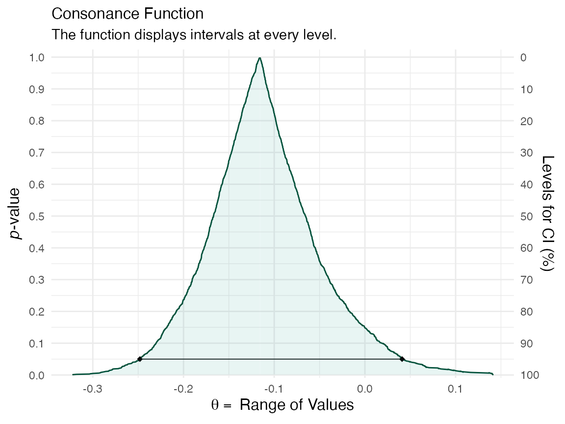
The first item in the list will be the consonance distribution constructed by typical means, while the third item will be the bootstrap approximation to the consonance distribution.

ggcurve(data = y[[1]], nullvalue = TRUE)

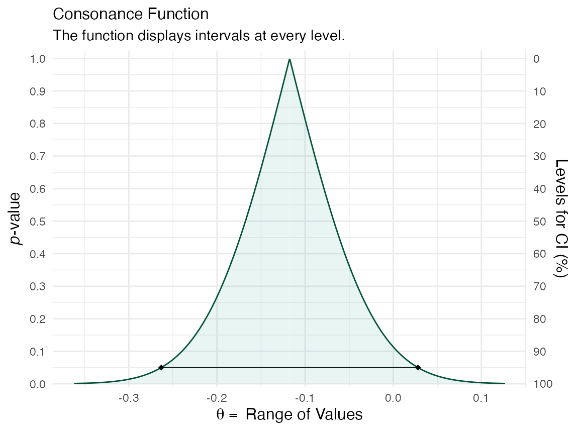
ggcurve(data = y[[3]], nullvalue = TRUE)

We can also print out a table for TeX documents

(gg <- curve_table(data = y[[1]], format = "image"))

Lower Limit	Upper Limit	Interval Width	Interval Level (%)	CDF	P-value	S-value (bits)
-0.141	-0.094	0.047	25	0.625	0.75	0.415
-0.168	-0.067	0.100	50	0.750	0.50	1.000
-0.203	-0.032	0.171	75	0.875	0.25	2.000
-0.213	-0.022	0.190	80	0.900	0.20	2.322
-0.263	0.028	0.291	95	0.975	0.05	4.322
-0.309	0.074	0.383	99	0.995	0.01	6.644

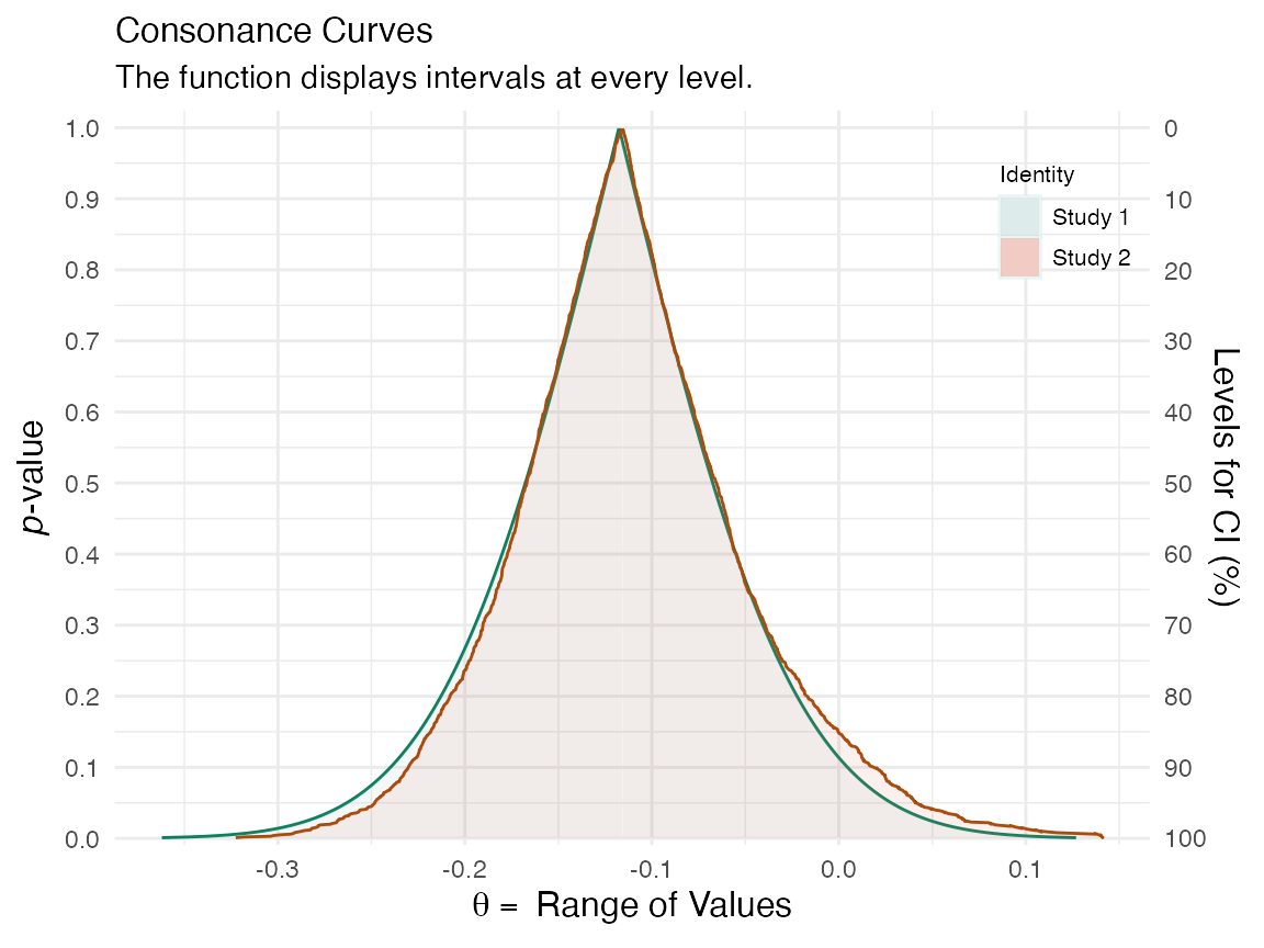
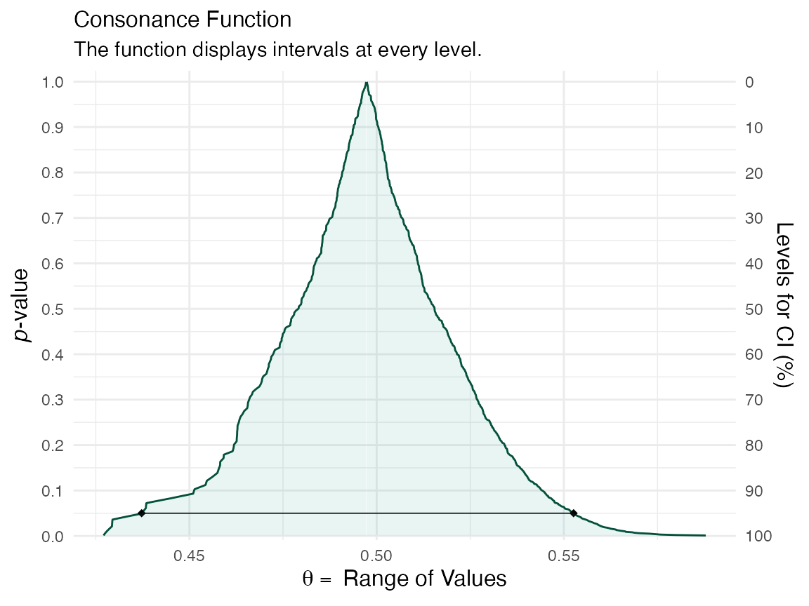
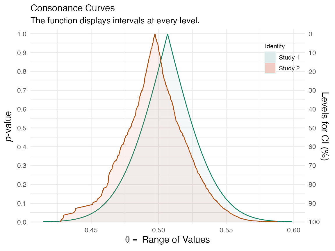
More bootstrap replications will lead to a smoother function. But for now, we can compare these two functions to see how similar they are.

plot_compare(y[[1]], y[[3]])

If we wanted to look at the bootstrap standard errors, we could do so by loading the fifth item in the list

knitr::kable(y[[5]])

	theta	sdboot	z0	a	sdjack
est	-0.1175698	0.0742970	0.0150403	0.0304863	0.075694
jsd	0.0000000	0.0013055	0.0308530	0.0000000	0.000000

where in the top row, theta is the point estimate, and sdboot is the bootstrap estimate of the standard error, sdjack is the jacknife estimate of the standard error. z0 is the bias correction value and a is the acceleration constant.

The values in the second row are essentially the internal standard errors of the estimates in the top row.

---

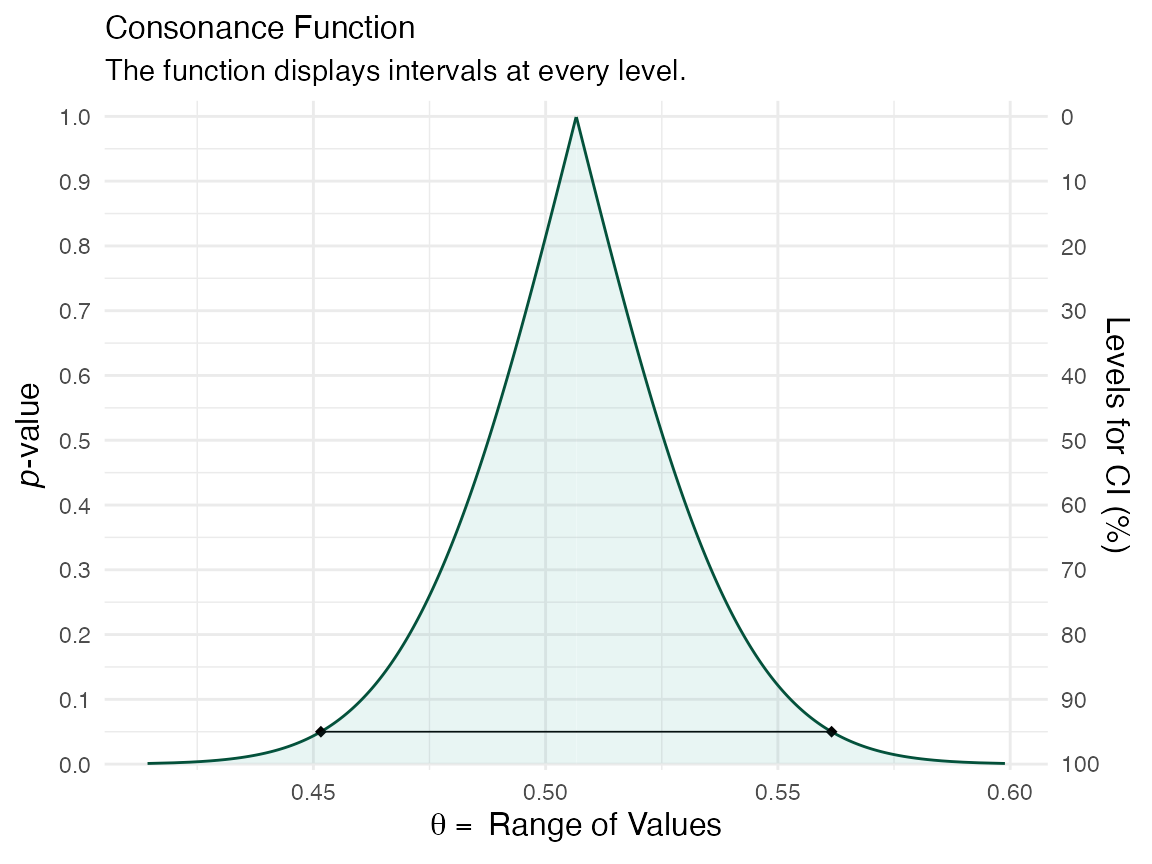
The densities can also be calculated accurately using the t-bootstrap method. Here we use a different dataset to show this

library(Lock5Data)
dataz <- data(CommuteAtlanta)
func <- function(data, index) {
  x <- as.numeric(unlist(data[1]))
  y <- as.numeric(unlist(data[2]))
  return(mean(x[index]) - mean(y[index]))
}

Our function is a simple mean difference. This time, we’ll set the method to “t” for the t-bootstrap method

z <- curve_boot(data = CommuteAtlanta, func = func, method = "t", replicates = 2000, steps = 1000)
#> Warning in norm.inter(t, alpha): extreme order statistics used as endpoints
ggcurve(data = z[[1]], nullvalue = FALSE)

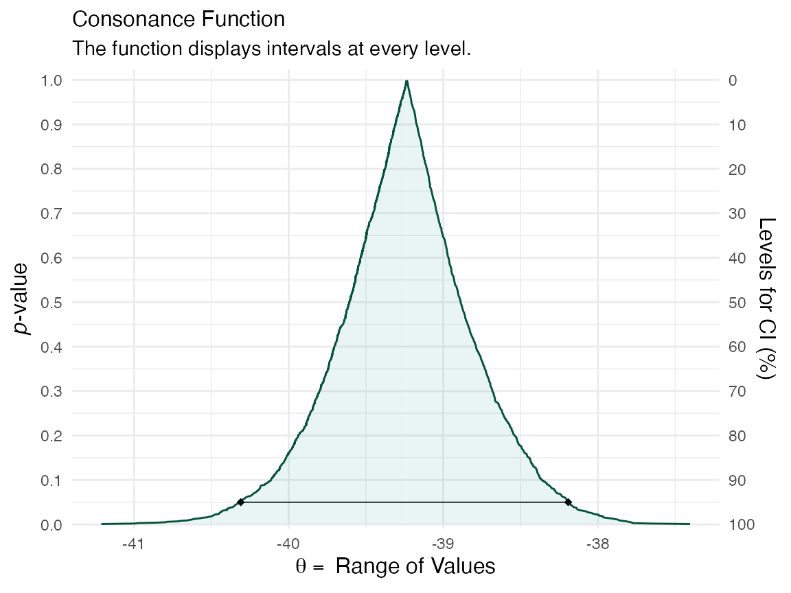
ggcurve(data = z[[2]], type = "cd", nullvalue = FALSE)

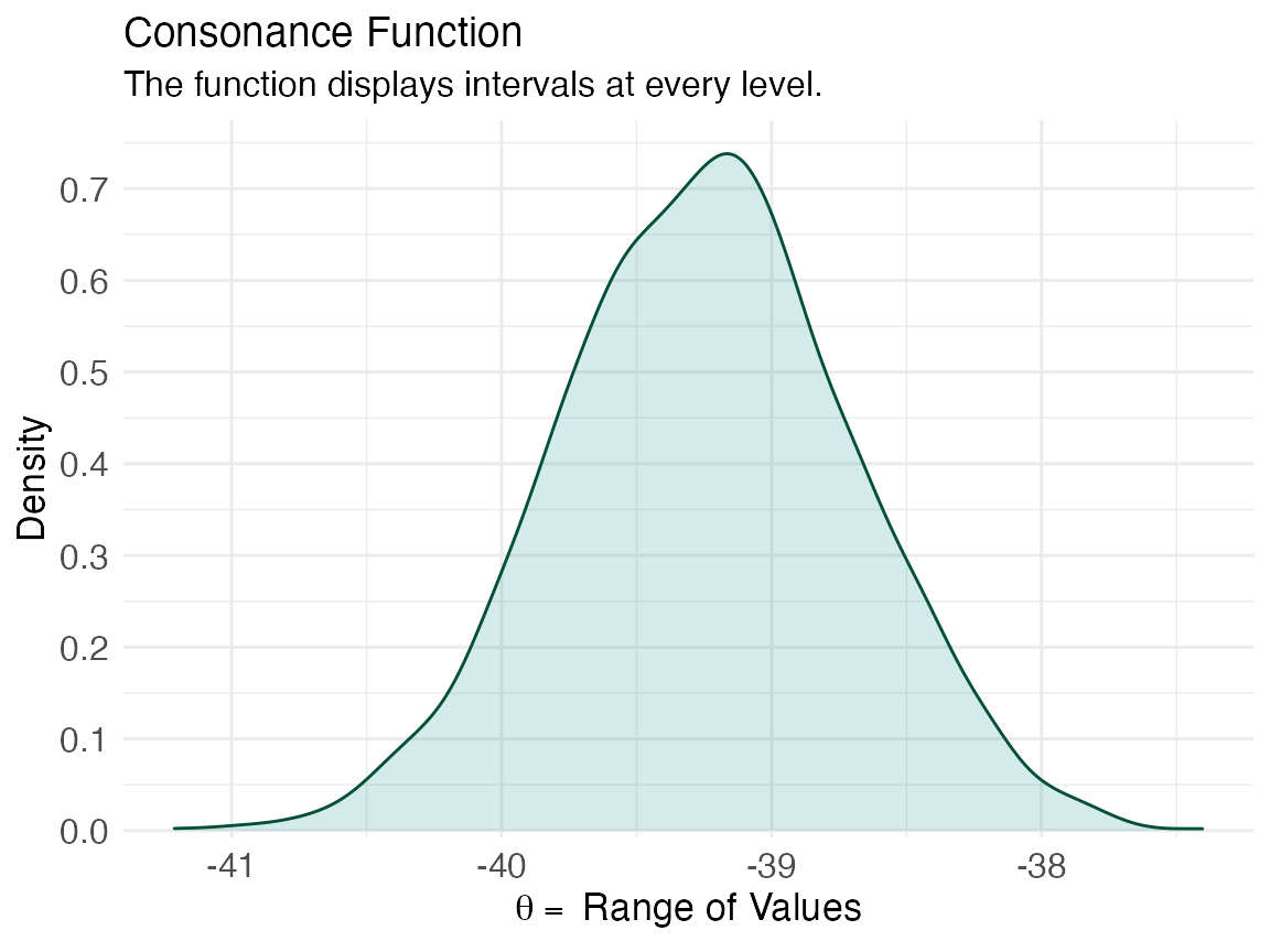
The consonance curve and density are nearly identical. With more bootstrap replications, they are very likely to converge.

(zz <- curve_table(data = z[[1]], format = "image"))

Lower Limit	Upper Limit	Interval Width	Interval Level (%)	CDF	P-value	S-value (bits)
-39.416	-39.076	0.340	25.0	0.625	0.750	0.415
-39.608	-38.888	0.720	50.0	0.750	0.500	1.000
-39.862	-38.616	1.245	75.0	0.875	0.250	2.000
-39.938	-38.540	1.398	80.0	0.900	0.200	2.322
-40.016	-38.443	1.573	85.0	0.925	0.150	2.737
-40.114	-38.360	1.754	90.0	0.950	0.100	3.322
-40.310	-38.192	2.118	95.0	0.975	0.050	4.322
-40.450	-38.036	2.414	97.5	0.988	0.025	5.322
-40.642	-37.866	2.776	99.0	0.995	0.010	6.644

The Parametric Bootstrap

For the examples above, we mainly used nonparametric bootstrap methods. Here I show an example using the parametric Bca bootstrap and the results it yields.

First, we’ll load our data again and set our function.

data(diabetes, package = "bcaboot")
X <- diabetes$x
y <- scale(diabetes$y, center = TRUE, scale = FALSE)
lm.model <- lm(y ~ X - 1)
mu.hat <- lm.model$fitted.values
sigma.hat <- stats::sd(lm.model$residuals)
t0 <- summary(lm.model)$adj.r.squared
y.star <- sapply(mu.hat, rnorm, n = 1000, sd = sigma.hat)
tt <- apply(y.star, 1, function(y) summary(lm(y ~ X - 1))$adj.r.squared)
b.star <- y.star %*% X

Now, we’ll use the same function, but set the method to “bcapar” for the parametric method.

df <- curve_boot(method = "bcapar", t0 = t0, tt = tt, bb = b.star)

Now we can look at our outputs.

ggcurve(df[[1]], nullvalue = FALSE)

ggcurve(df[[3]], nullvalue = FALSE)

We can compare the functions to see how well the bootstrap approximations match up

plot_compare(df[[1]], df[[3]])

That concludes our demonstration of the bootstrap method to approximate consonance functions.

Cite R Packages

Please remember to cite the packages that you use.

citation("concurve")
#> 
#> Rafi Z, Vigotsky A (2020). _concurve: Computes and Plots Compatibility
#> (Confidence) Intervals, P-Values, S-Values, & Likelihood Intervals to
#> Form Consonance, Surprisal, & Likelihood Functions_. R package version
#> 2.7.7, <URL: https://CRAN.R-project.org/package=concurve>.
#> 
#> Rafi Z, Greenland S (2020). "Semantic and Cognitive Tools to Aid
#> Statistical Science: Replace Confidence and Significance by
#> Compatibility and Surprise." _BMC Medical Research Methodology_, *20*,
#> 244. ISSN 1471-2288, doi: 10.1186/s12874-020-01105-9 (URL:
#> https://doi.org/10.1186/s12874-020-01105-9), <URL:
#> https://doi.org/10.1186/s12874-020-01105-9>.
#> 
#> To see these entries in BibTeX format, use 'print(<citation>,
#> bibtex=TRUE)', 'toBibtex(.)', or set
#> 'options(citation.bibtex.max=999)'.
citation("boot")
#> 
#> To cite the 'boot' package in publications use:
#> 
#>   Angelo Canty and Brian Ripley (2020). boot: Bootstrap R (S-Plus)
#>   Functions. R package version 1.3-25.
#> 
#>   Davison, A. C. & Hinkley, D. V. (1997) Bootstrap Methods and Their
#>   Applications. Cambridge University Press, Cambridge. ISBN
#>   0-521-57391-2
#> 
#> To see these entries in BibTeX format, use 'print(<citation>,
#> bibtex=TRUE)', 'toBibtex(.)', or set
#> 'options(citation.bibtex.max=999)'.
citation("bcaboot")
#> 
#> To cite package 'bcaboot' in publications use:
#> 
#>   Bradley Efron and Balasubramanian Narasimhan (2018). bcaboot: Bias
#>   Corrected Bootstrap Confidence Intervals. R package version 0.2-1.
#>   https://CRAN.R-project.org/package=bcaboot
#> 
#> A BibTeX entry for LaTeX users is
#> 
#>   @Manual{,
#>     title = {bcaboot: Bias Corrected Bootstrap Confidence Intervals},
#>     author = {Bradley Efron and Balasubramanian Narasimhan},
#>     year = {2018},
#>     note = {R package version 0.2-1},
#>     url = {https://CRAN.R-project.org/package=bcaboot},
#>   }

---

References

---

1. Efron B. R. A. Fisher in the 21st century (Invited paper presented at the 1996 R. A. Fisher Lecture). Statistical Science. 1998;13(2):95-122. doi:10/cxg354

2. Efron B, Narasimhan B. The automatic construction of bootstrap confidence intervals. October 2018:17.

3. Xie M-g, Singh K. Confidence Distribution, the Frequentist Distribution Estimator of a Parameter: A Review. International Statistical Review. 2013;81(1):3-39. doi:10.1111/insr.12000