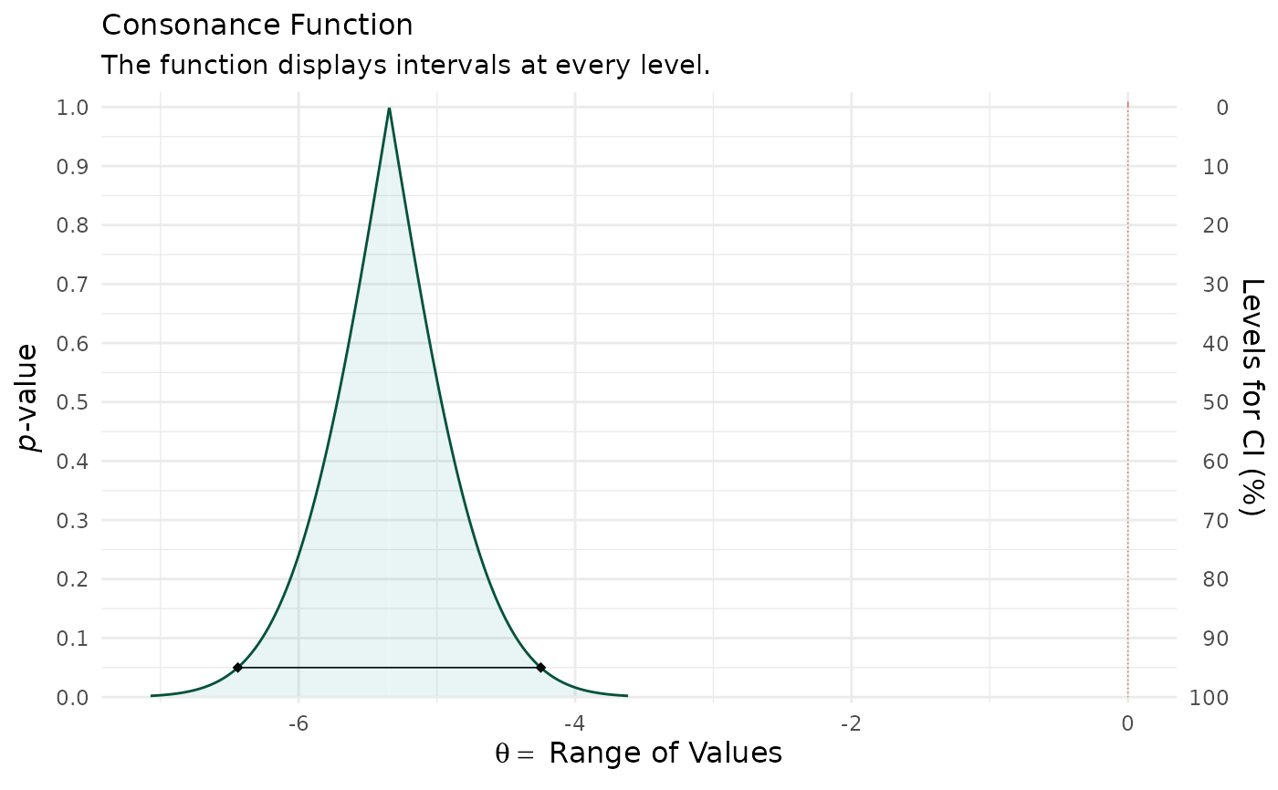
Takes the dataframe produced by the interval functions and plots the p-values/s-values, consonance (confidence) levels, and the interval estimates to produce a p-value/s-value function using ggplot2 graphics.
ggcurve(data, type = c("c", "s", "cdf", "cd", "l1", "l2", "l3", "d"),
  measure = c("default", "ratio"), levels = 0.95, nullvalue = NULL,
  position = c("pyramid", "inverted"), title = "Consonance Function",
  subtitle = "The function displays intervals at every level.",
  xaxis = expression(theta == ~"Range of Values"),
  yaxis1 = expression(paste(italic(p), "-value")),
  yaxis2 = "Levels for CI (%)", color = colorspace::darken("#009E73",
  0.5), fill = "#239a98")
Arguments
- data
The dataframe produced by one of the interval functions in which the intervals are stored.
- type
The kind of function to plot. One of
"c"for a consonance function, the default,"s"for a surprisal function,"cdf"for the consonance distribution function,"cd"for the consonance density function,"l1"for relative likelihood,"l2"for log-likelihood,"l3"for likelihood, or"d"for the deviance function. An unrecognized value is an error naming the permitted ones.- measure
Indicates whether the object has a log transformation or is normal/default. The default setting is "default". If the measure is set to "ratio", it will take logarithmically transformed values and convert them back to normal values in the dataframe. This is typically a setting used for binary outcomes and their measures such as risk ratios, hazard ratios, and odds ratios.
- levels
Indicates which interval levels should be plotted on the function. By default it is set to 0.95 to plot the 95% interval on the consonance function, but more levels can be plotted by using the c() function for example, levels = c(0.50, 0.75, 0.95).
- nullvalue
Indicates whether the null value for the measure should be plotted. By default, it is set to NULL, meaning it will not be plotted as a vertical line. Changing this to a numerical vector will specify the region where a line should be plotted or an area that should be shaded. The input must be a numerical vector, for example c(-0.5, 0.5) or a single numerical vector such as 0 or 1.
- position
Determines the orientation of the P-value (consonance) function. By default, it is set to "pyramid", meaning the p-value function will stand right side up, like a pyramid. However, it can also be inverted via the option "inverted". This will also change the sequence of the y-axes to match the orientation.This can be set as such, ggcurve(type = "c", data = df, position = "inverted").
- title
A custom title for the graph. By default, it is set to "Consonance Function". In order to set a title, it must be in quotes. For example, ggcurve(type = "c", data = x, title = "Custom Title").
- subtitle
A custom subtitle for the graph. By default, it is set to "The function contains consonance/confidence intervals at every level and the P-values." In order to set a subtitle, it must be in quotes. For example, ggcurve(type = "c", data = x, subtitle = "Custom Subtitle").
- xaxis
A custom x-axis title for the graph. By default, it is set to "Range of Values. In order to set a x-axis title, it must be in quotes. For example, ggcurve(type = "c", data = x, xaxis = "Hazard Ratio").
- yaxis1
A custom y-axis title for the graph. By default, it is set to "Consonance Level". In order to set a y-axis title, it must be in quotes. For example, ggcurve(type = "c", data = x, yxis1= "Confidence Level").
- yaxis2
A custom y-axis title for the graph. By default, it is set to "Levels for CI". In order to set a y-axis title, it must be in quotes. For example, ggcurve(type = "c", data = x, yxis2= "Confidence Level").
- color
Item that allows the user to choose the color of the points and the ribbons in the graph. By default, it is set to color = "#555555". The inputs must be in quotes. For example, ggcurve(type = "c", data = x, color = "#333333").
- fill
Item that allows the user to choose the color of the ribbons in the graph. By default, it is set to fill = "#239a98". The inputs must be in quotes. For example, ggcurve(type = "c", data = x, fill = "#333333").
Value
A plot with intervals at every consonance level graphed with their corresponding p-values and compatibility levels.
See also
Examples
# The consonance curve for a regression coefficient. Every horizontal
# slice is an interval, and the height is the P-value for that value
# of the parameter.
curves <- curve_gen(lm(mpg ~ wt, data = mtcars), "wt")
ggcurve(curves[[1]], type = "c", nullvalue = 0)
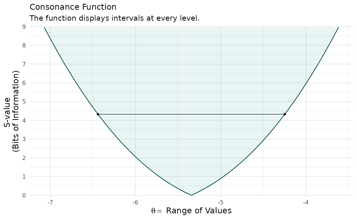
 # The same evidence as surprisal, -log2(p): the bits of information
# against each value. The 95% limits sit at about 4.3 bits.
ggcurve(curves[[1]], type = "s")
# The same evidence as surprisal, -log2(p): the bits of information
# against each value. The 95% limits sit at about 4.3 bits.
ggcurve(curves[[1]], type = "s")
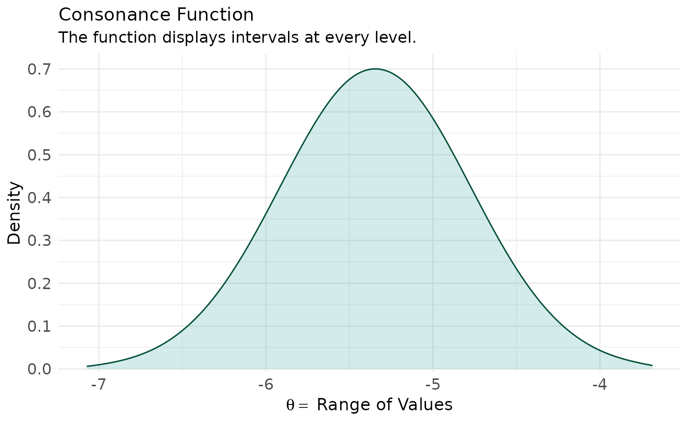
 # The consonance density, built from the second element of the object
ggcurve(curves[[2]], type = "cd")
# The consonance density, built from the second element of the object
ggcurve(curves[[2]], type = "cd")
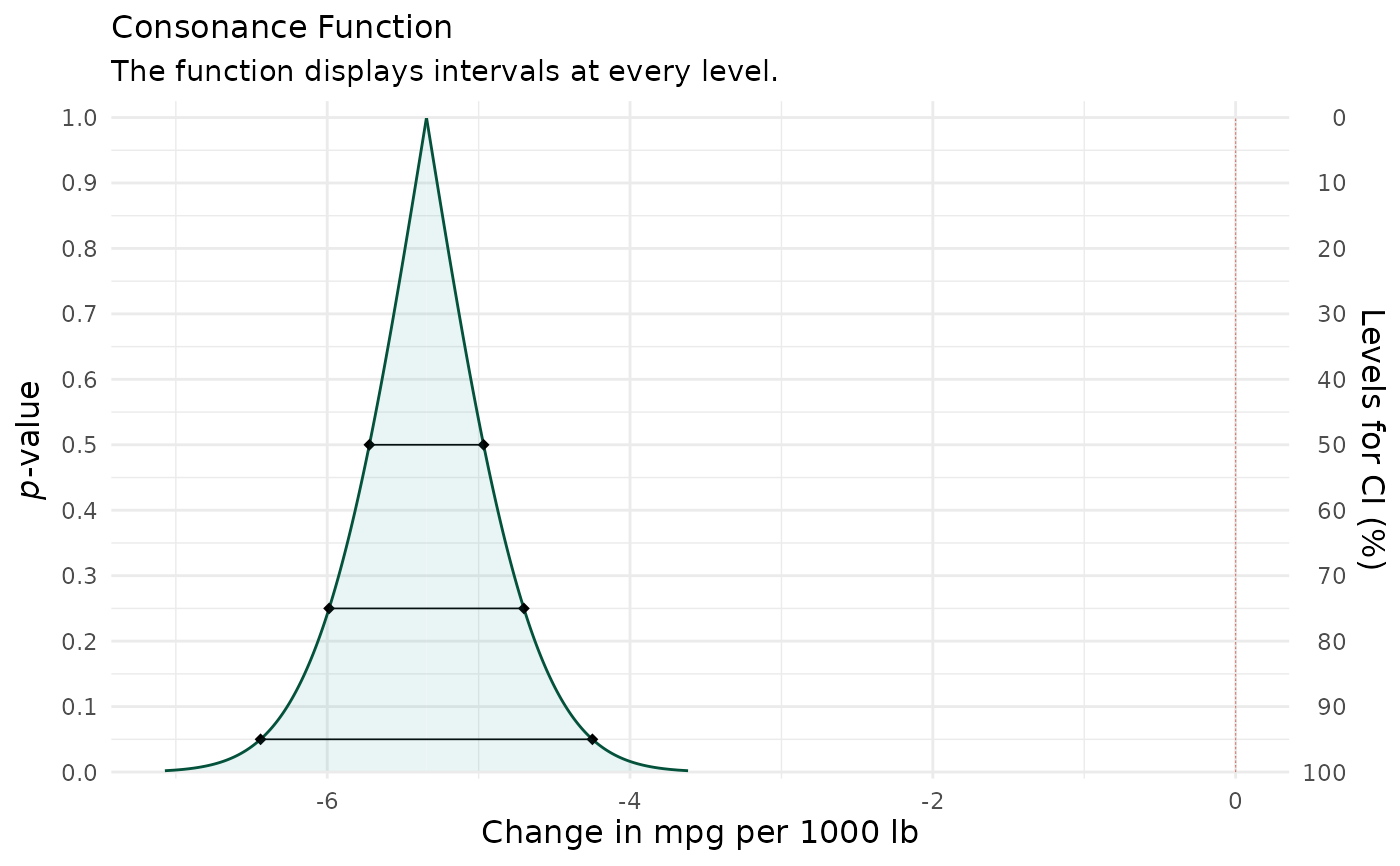
 # Several interval levels at once, with a relabelled axis
ggcurve(
curves[[1]],
type = "c",
levels = c(0.50, 0.75, 0.95),
nullvalue = 0,
xaxis = "Change in mpg per 1000 lb"
)
# Several interval levels at once, with a relabelled axis
ggcurve(
curves[[1]],
type = "c",
levels = c(0.50, 0.75, 0.95),
nullvalue = 0,
xaxis = "Change in mpg per 1000 lb"
)