Suppose we wanted to produce confidence distributions for data with binary outcomes and where we employ a logistic regression, we would do the following. Here, I use the mtcars dataset for the example and also simulate some very simple binary data. We use suppressMessages() to avoid seeing the long list of profiling messages.
## Please see the documentation on https://data.lesslikely.com/concurve/ or by typing `help(concurve)`X <- rnorm(100, mean = 0, sd = 1) Y <- rbinom(n = 100, size = 1, prob = 0.5) mydata1 <- data.frame(X, Y) model1 <- glm(Y ~ X, data = mydata1, family = binomial(link = "logit")) model2 <- glm(am ~ mpg, family = binomial(link = "logit"), data = mtcars) summary(model1)
##
## Call:
## glm(formula = Y ~ X, family = binomial(link = "logit"), data = mydata1)
##
## Deviance Residuals:
##    Min      1Q  Median      3Q     Max
## -1.459  -1.136  -0.889   1.167   1.497
##
## Coefficients:
##             Estimate Std. Error z value Pr(>|z|)
## (Intercept) -0.02064    0.20301  -0.102    0.919
## X            0.35394    0.22524   1.571    0.116
##
## (Dispersion parameter for binomial family taken to be 1)
##
##     Null deviance: 138.59  on 99  degrees of freedom
## Residual deviance: 136.02  on 98  degrees of freedom
## AIC: 140.02
##
## Number of Fisher Scoring iterations: 4summary(model2)
##
## Call:
## glm(formula = am ~ mpg, family = binomial(link = "logit"), data = mtcars)
##
## Deviance Residuals:
##     Min       1Q   Median       3Q      Max
## -1.5701  -0.7531  -0.4245   0.5866   2.0617
##
## Coefficients:
##             Estimate Std. Error z value Pr(>|z|)
## (Intercept)  -6.6035     2.3514  -2.808  0.00498 **
## mpg           0.3070     0.1148   2.673  0.00751 **
## ---
## Signif. codes:  0 '***' 0.001 '**' 0.01 '*' 0.05 '.' 0.1 ' ' 1
##
## (Dispersion parameter for binomial family taken to be 1)
##
##     Null deviance: 43.230  on 31  degrees of freedom
## Residual deviance: 29.675  on 30  degrees of freedom
## AIC: 33.675
##
## Number of Fisher Scoring iterations: 5
model_pro <- suppressMessages(curve_gen( model = model1, var = "X", method = "glm", log = T, steps = 1000, table = TRUE)) model_con <- suppressMessages(curve_gen( model = model2, var = "mpg", method = "glm", log = T, steps = 1000, table = TRUE)) head(model_con[[1]], 10)
##    lower.limit upper.limit intrvl.width intrvl.level    cdf pvalue      svalue
## 1     1.359192    1.359581 0.0003887775        0.001 0.5005  0.999 0.001443417
## 2     1.358998    1.359776 0.0007775530        0.002 0.5010  0.998 0.002888279
## 3     1.358804    1.359970 0.0011663270        0.003 0.5015  0.997 0.004334590
## 4     1.358609    1.360164 0.0015551002        0.004 0.5020  0.996 0.005782353
## 5     1.358415    1.360359 0.0019438731        0.005 0.5025  0.995 0.007231569
## 6     1.358221    1.360556 0.0023349563        0.006 0.5030  0.994 0.008682243
## 7     1.358027    1.360754 0.0027268373        0.007 0.5035  0.993 0.010134377
## 8     1.357833    1.360951 0.0031187240        0.008 0.5040  0.992 0.011587974
## 9     1.357638    1.361149 0.0035106173        0.009 0.5045  0.991 0.013043037
## 10 1.357444 1.361347 0.0039025176 0.010 0.5050 0.990 0.014499570(ggcurve(model_con[[1]], measure = "ratio", type = "c", nullvalue = c(0.8, 1.2), title = "Confidence Curve", subtitle = "The function displays intervals at every level.", xaxis = expression(theta == ~"Range of Values"), yaxis1 = expression(paste(italic(p), "-value")), yaxis2 = "Levels for CI (%)"))
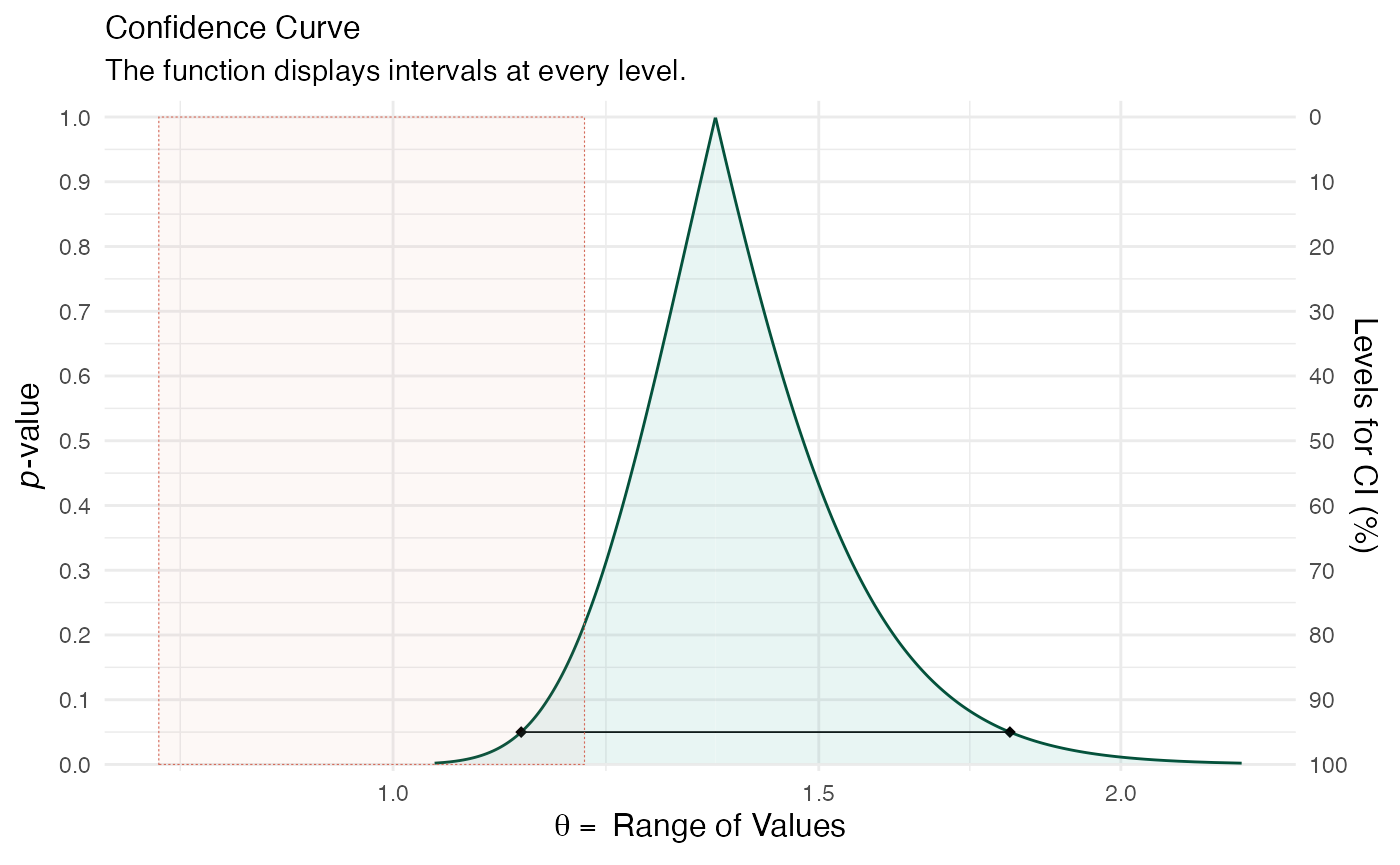
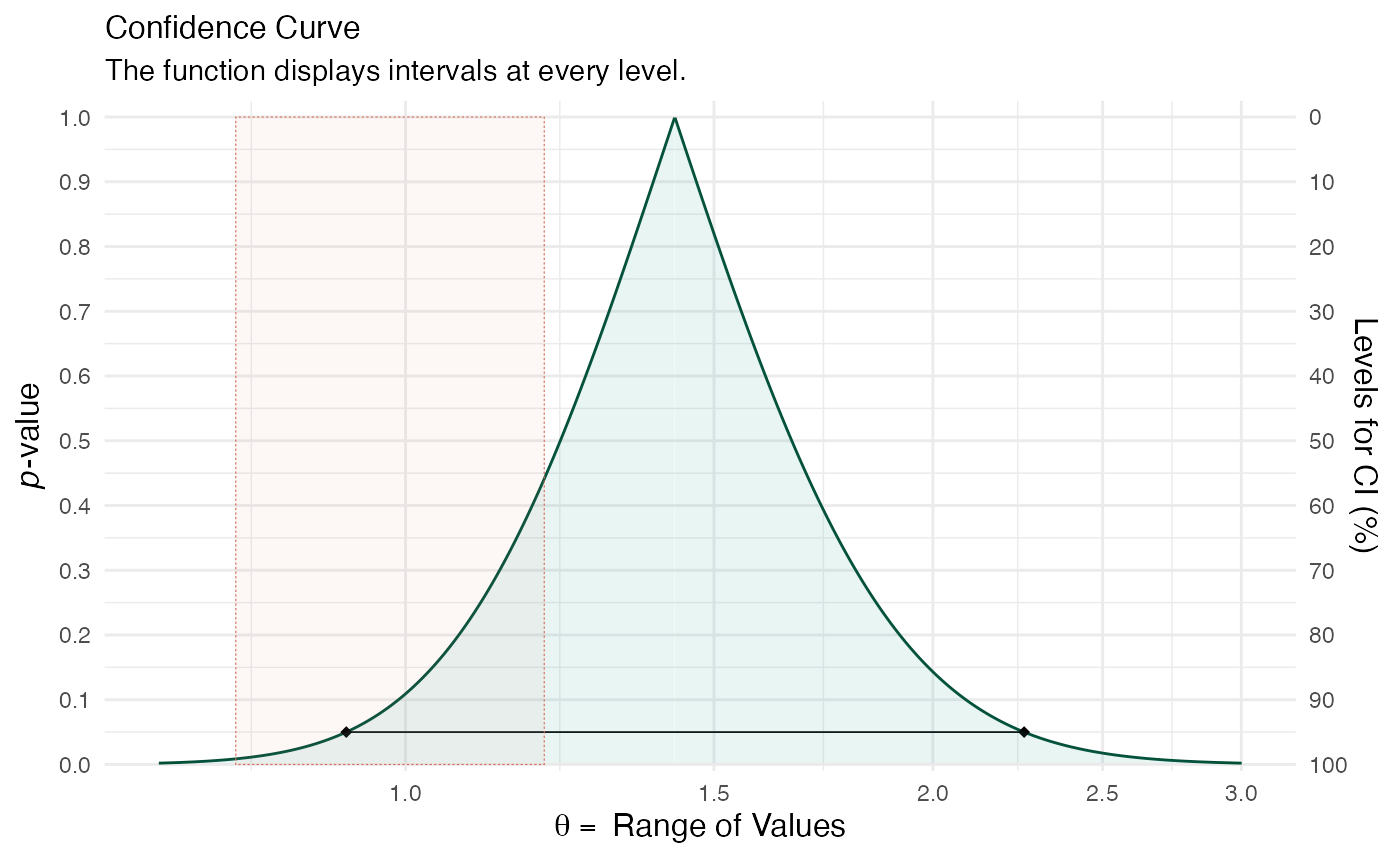
(ggcurve(model_pro[[1]],
    measure = "ratio",
    type = "c",
    nullvalue = c(0.8, 1.2), title = "Confidence Curve",
    subtitle = "The function displays intervals at every level.",
    xaxis = expression(theta == ~"Range of Values"),
    yaxis1 = expression(paste(italic(p), "-value")),
    yaxis2 = "Levels for CI (%)"))
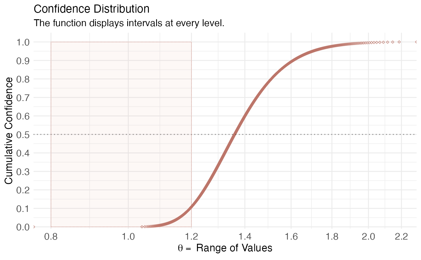
(ggcurve(model_con[[2]],
    measure = "ratio",
    type = "cdf",
    nullvalue = c(0.8, 1.2), title = "Confidence Distribution",
    subtitle = "The function displays intervals at every level.",
    xaxis = expression(theta == ~"Range of Values"),
    yaxis1 = expression(paste(italic(p), "-value")),
    yaxis2 = "Levels for CI (%)"))
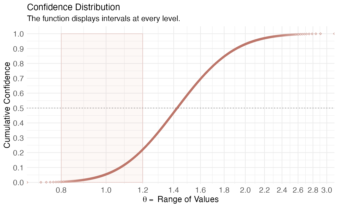
(ggcurve(model_pro[[2]],
    measure = "ratio",
    type = "cdf",
    nullvalue = c(0.8, 1.2), title = "Confidence Distribution",
    subtitle = "The function displays intervals at every level.",
    xaxis = expression(theta == ~"Range of Values"),
    yaxis1 = expression(paste(italic(p), "-value")),
    yaxis2 = "Levels for CI (%)"))
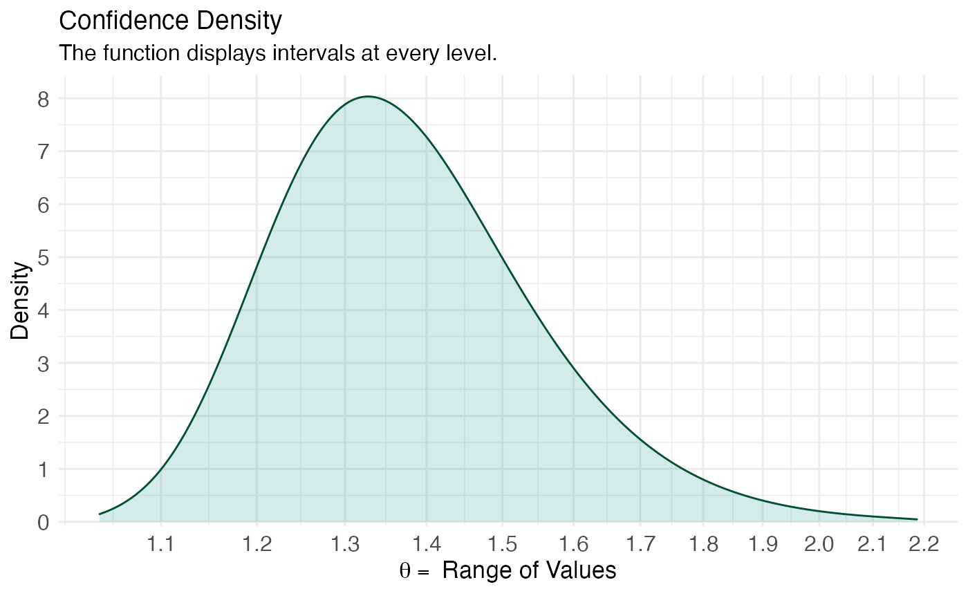
(ggcurve(model_con[[2]],
    measure = "ratio",
    type = "cd",
    nullvalue = NULL, title = "Confidence Density",
    subtitle = "The function displays intervals at every level.",
    xaxis = expression(theta == ~"Range of Values"),
    yaxis1 = expression(paste(italic(p), "-value")),
    yaxis2 = "Levels for CI (%)"))
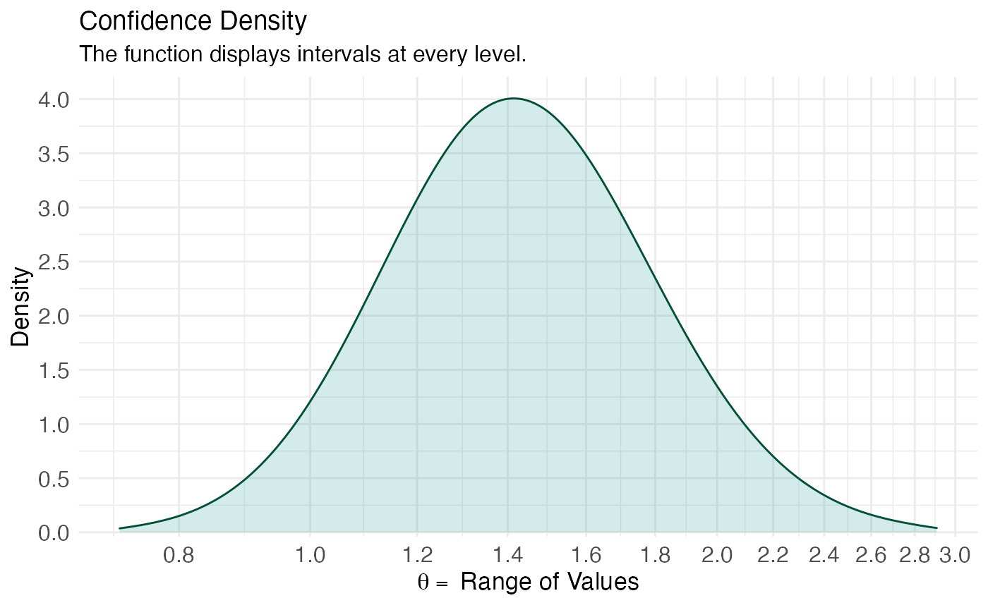
(ggcurve(model_pro[[2]],
    measure = "ratio",
    type = "cd",
    nullvalue = NULL, title = "Confidence Density",
    subtitle = "The function displays intervals at every level.",
    xaxis = expression(theta == ~"Range of Values"),
    yaxis1 = expression(paste(italic(p), "-value")),
    yaxis2 = "Levels for CI (%)"))
Cite R Packages
Please remember to cite the R packages that you use in your work.
citation("concurve")
##
## Rafi Z, Vigotsky A (2020). _concurve: Computes and Plots Compatibility
## (Confidence) Intervals, P-Values, S-Values, & Likelihood Intervals to
## Form Consonance, Surprisal, & Likelihood Functions_. R package version
## 2.7.7, <URL: https://CRAN.R-project.org/package=concurve>.
##
## Rafi Z, Greenland S (2020). "Semantic and Cognitive Tools to Aid
## Statistical Science: Replace Confidence and Significance by
## Compatibility and Surprise." _BMC Medical Research Methodology_, *20*,
## 244. ISSN 1471-2288, doi: 10.1186/s12874-020-01105-9 (URL:
## https://doi.org/10.1186/s12874-020-01105-9), <URL:
## https://doi.org/10.1186/s12874-020-01105-9>.
##
## To see these entries in BibTeX format, use 'print(<citation>,
## bibtex=TRUE)', 'toBibtex(.)', or set
## 'options(citation.bibtex.max=999)'.citation("cowplot")
##
## To cite package 'cowplot' in publications use:
##
##   Claus O. Wilke (2020). cowplot: Streamlined Plot Theme and Plot
##   Annotations for 'ggplot2'. R package version 1.1.0.
##   https://CRAN.R-project.org/package=cowplot
##
## A BibTeX entry for LaTeX users is
##
##   @Manual{,
##     title = {cowplot: Streamlined Plot Theme and Plot Annotations for 'ggplot2'},
##     author = {Claus O. Wilke},
##     year = {2020},
##     note = {R package version 1.1.0},
##     url = {https://CRAN.R-project.org/package=cowplot},
##   }