Count and Rate Models: Likelihood and P-value Functions • concurve

Count outcomes — events per person, per unit time, per unit area — are the natural home of the Poisson model, and the parameter that epidemiologists actually care about is the rate ratio.¹ This vignette leads with the likelihood function for a Poisson log-rate-ratio and then shows the matching consonance (P-value) function, so you can see the same coefficient described two ways.^2,3

The data

We simulate counts for an exposed vs. unexposed group, adjusting for one continuous covariate. The true log-rate-ratio for group is $0.8$ (a rate ratio of about $2.2$ ).

set.seed(2718)
n <- 200
x1    <- rnorm(n)
group <- rbinom(n, size = 1, prob = 0.5)
eta   <- -0.5 + 0.8 * group + 0.3 * x1
y     <- rpois(n, lambda = exp(eta))

pois_dat <- data.frame(y, group, x1)
head(pois_dat)
#>   y group         x1
#> 1 0     0  0.4851789
#> 2 0     0 -1.1725243
#> 3 2     1  0.6890232
#> 4 1     0 -0.6219502
#> 5 0     1 -0.7274038
#> 6 1     0 -0.6131067

Constructing the likelihood function

We reuse the same machinery as the profile-likelihood vignette: ProfileLikelihood::profilelike.glm() profiles the Poisson GLM over the nuisance coefficients at each value of the target parameter, and curve_lik() turns that into a concurve likelihood object.^4,5 The variable named in profile.theta (here group) is the one profiled; it is left out of the formula.

library(ProfileLikelihood)

xx <- profilelike.glm(
  y ~ x1,
  data          = pois_dat,
  profile.theta = "group",
  family        = poisson(link = "log"),
  length        = 500,
  round         = 2
)
#> Warning message: provide lo.theta and hi.theta

lik <- curve_lik(xx, data = pois_dat)

The profiled parameter is on the log scale, so values here are candidate log-rate-ratios and the null of “no association” is at $0$ .

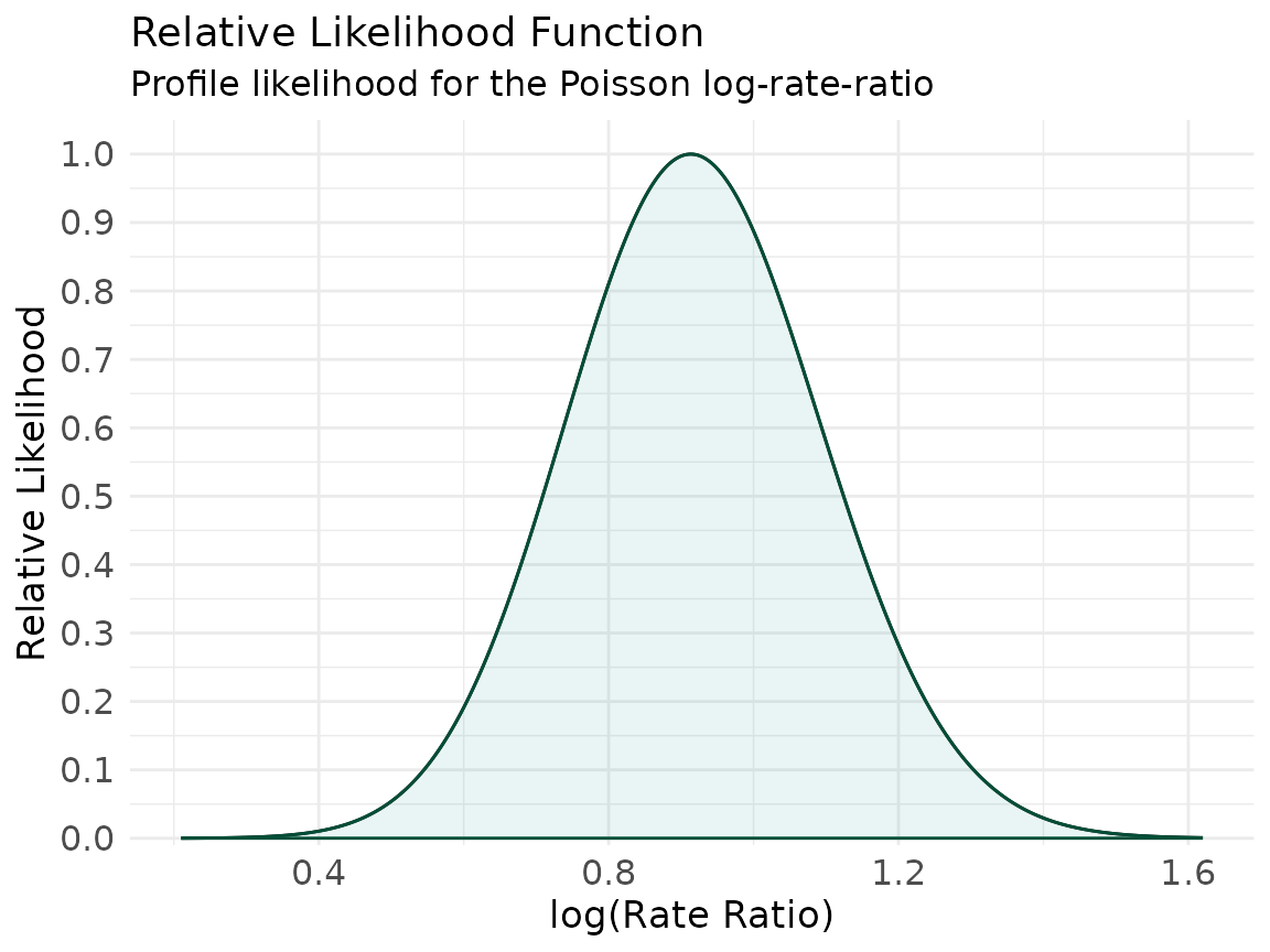
Plotting the likelihood

ggcurve(lik[[1]], type = "l1", nullvalue = TRUE,
        xaxis = "log(Rate Ratio)",
        title = "Relative Likelihood Function",
        subtitle = "Profile likelihood for the Poisson log-rate-ratio")


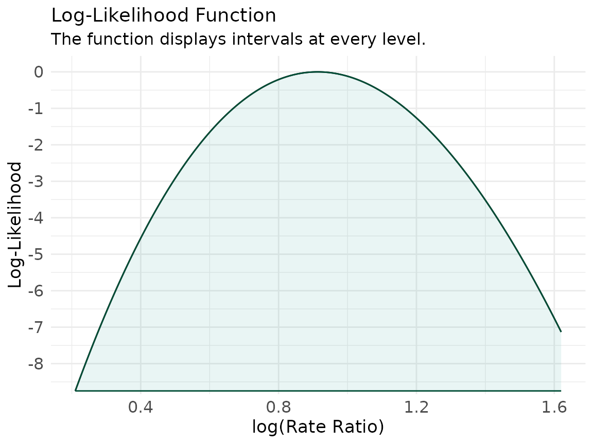
ggcurve(lik[[1]], type = "l2",
        xaxis = "log(Rate Ratio)",
        title = "Log-Likelihood Function")


ggcurve(lik[[1]], type = "d", nullvalue = 0,
        xaxis = "log(Rate Ratio)",
        title = "Deviance Function")
#> Warning: Using `size` aesthetic for lines was deprecated in ggplot2 3.4.0.
#> ℹ Please use `linewidth` instead.
#> ℹ The deprecated feature was likely used in the concurve package.
#>   Please report the issue at <https://github.com/zadrafi/concurve/issues>.
#> This warning is displayed once per session.
#> Call `lifecycle::last_lifecycle_warnings()` to see where this warning was
#> generated.

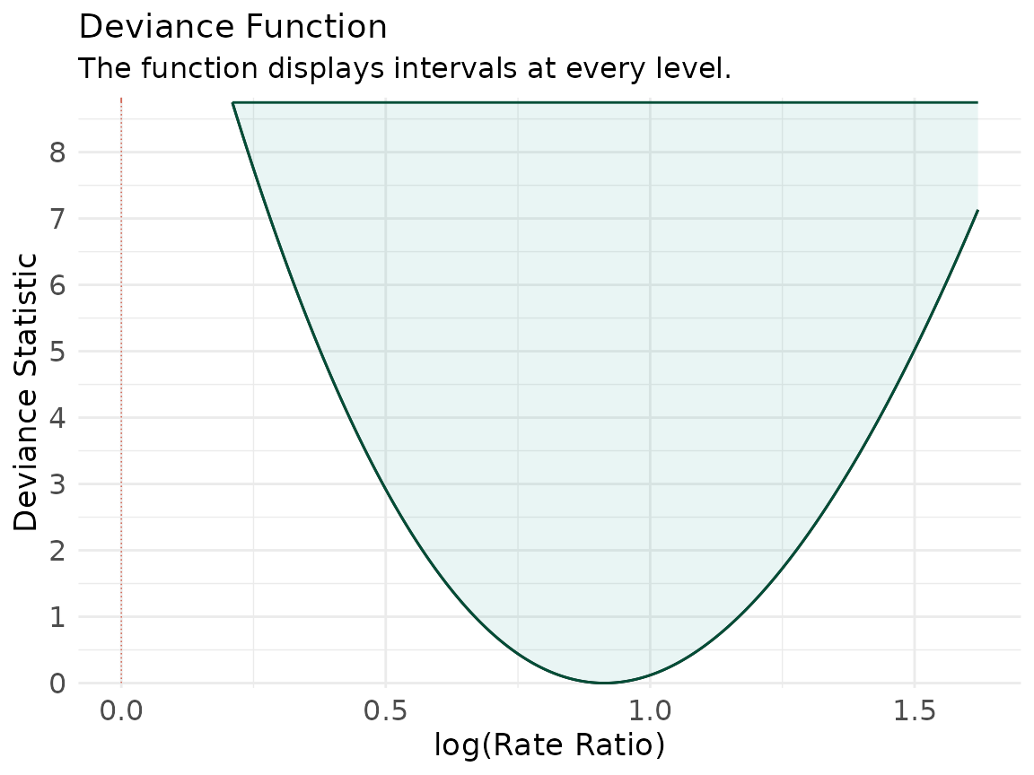
The likelihood peaks near the true value of $0.8$ , and the deviance function — $-\log$ relative likelihood — turns the same curve into a “distance from the best-supported value” scale, where Royall’s $1/8$ and $1/32$ support cutoffs correspond to deviance heights of about $2.08$ and $3.47$ .⁶

The companion: consonance and surprisal functions

For the frequentist view we fit the full Poisson GLM and hand it to curve_gen() with method = "glm". Setting log = TRUE keeps the underlying values on the log scale but lets us plot on the rate-ratio scale with measure = "ratio", where the null is $1$ .² We wrap the call in suppressMessages() to hide the long list of profiling messages.

pois_mod <- glm(y ~ group + x1, data = pois_dat, family = poisson(link = "log"))

rate_curve <- suppressMessages(curve_gen(
  model  = pois_mod,
  var    = "group",
  method = "glm",
  log    = TRUE,
  steps  = 1000
))

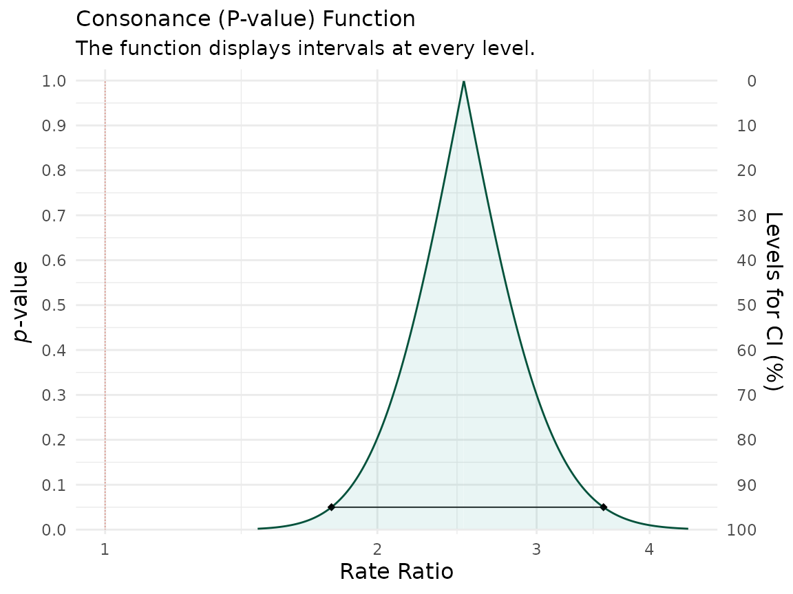
ggcurve(rate_curve[[1]], type = "c", measure = "ratio", nullvalue = 1,
        xaxis = "Rate Ratio",
        title = "Consonance (P-value) Function")


ggcurve(rate_curve[[1]], type = "s", measure = "ratio", nullvalue = 1,
        xaxis = "Rate Ratio",
        title = "Surprisal (S-value) Function")
#> Warning: Unknown or uninitialised column: `svalue`.
#> Unknown or uninitialised column: `svalue`.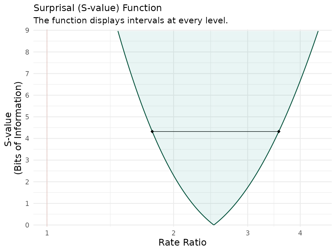

The consonance function peaks at the estimated rate ratio; its slice at $1 - \alpha = 0.95$ is the ordinary 95% rate-ratio interval. The surprisal function reports $-\log_2 p$ against each candidate rate ratio, so a rate ratio of $1$ carries a readable number of bits of information against it.^2,7

A confidence distribution too

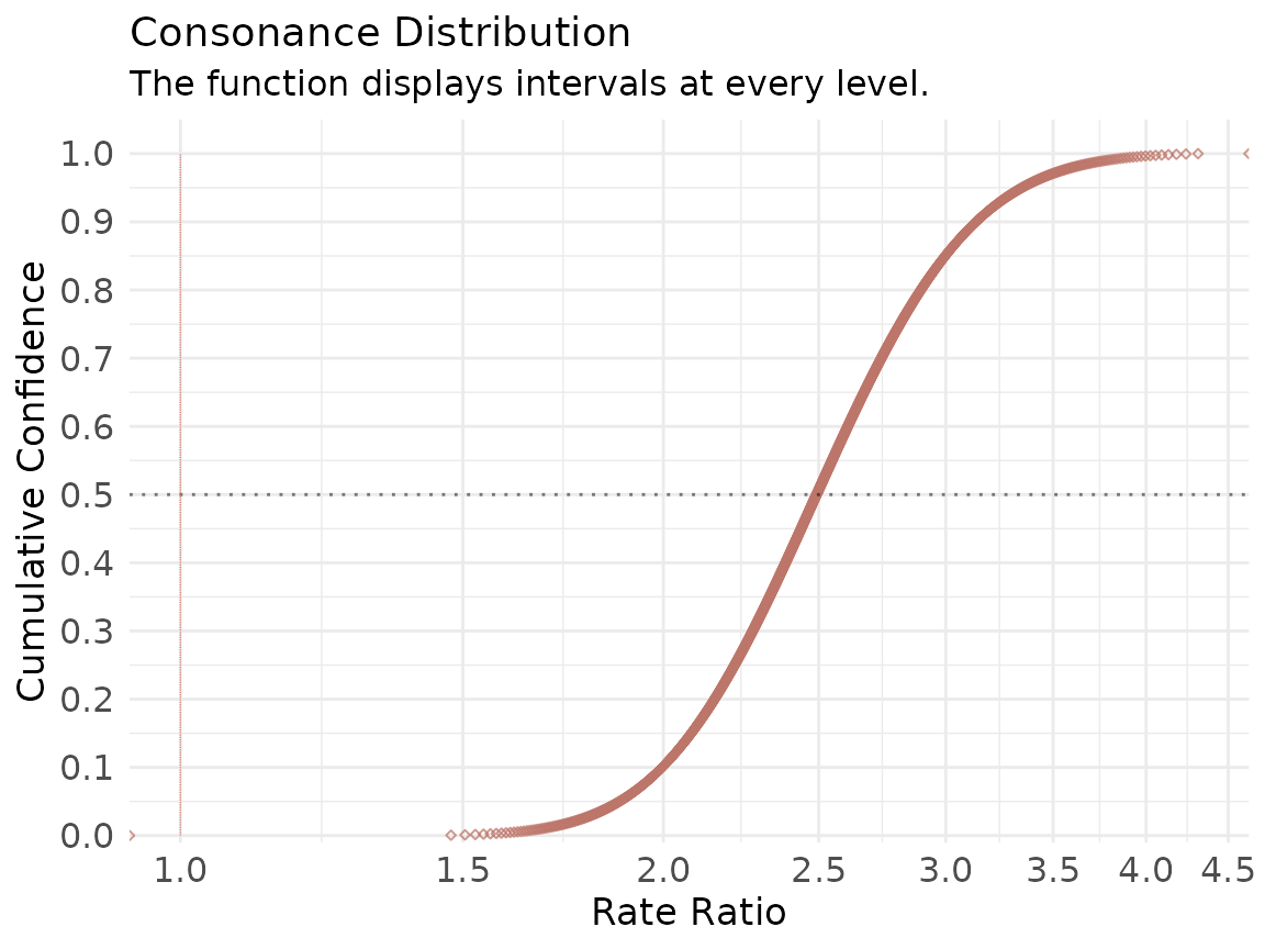
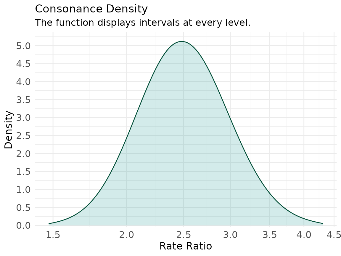
Because curve_gen() also returns the density-function values, you can draw the full confidence distribution and density for the rate ratio.^8,9

ggcurve(rate_curve[[2]], type = "cdf", measure = "ratio", nullvalue = 1,
        xaxis = "Rate Ratio",
        title = "Consonance Distribution")


ggcurve(rate_curve[[2]], type = "cd", measure = "ratio",
        xaxis = "Rate Ratio",
        title = "Consonance Density")

Putting it together

The log-rate-ratio likelihood and the rate-ratio consonance function are the same coefficient viewed on two scales and through two inferential lenses. The likelihood asks how well each value is supported by the data; the consonance function asks how compatible each value is under the model.² For a smooth one-parameter target like this, the $1/6.8$ likelihood interval and the 95% consonance interval will land in almost the same place — which is exactly why neither a single interval nor a single P-value deserves a bright line.¹⁰

Cite R Packages

Please remember to cite the packages that you use.

citation("concurve")
#> To cite package 'concurve' in publications use:
#> 
#>   Rafi Z, Vigotsky A (2026). _concurve: Computes and Plots
#>   Compatibility (Confidence) Intervals, P-Values, S-Values, &
#>   Likelihood Intervals to Form Consonance, Surprisal, & Likelihood
#>   Functions_. R package version 3.0.0,
#>   <https://CRAN.R-project.org/package=concurve>.
#> 
#>   Rafi Z, Greenland S (2020). "Semantic and Cognitive Tools to Aid
#>   Statistical Science: Replace Confidence and Significance by
#>   Compatibility and Surprise." _BMC Medical Research Methodology_,
#>   *20*, 244. ISSN 1471-2288. doi:10.1186/s12874-020-01105-9
#>   <https://doi.org/10.1186/s12874-020-01105-9>.
#>   <https://doi.org/10.1186/s12874-020-01105-9>.
#> 
#> To see these entries in BibTeX format, use 'print(<citation>,
#> bibtex=TRUE)', 'toBibtex(.)', or set
#> 'options(citation.bibtex.max=999)'.
citation("ProfileLikelihood")
#> To cite package 'ProfileLikelihood' in publications use:
#> 
#>   Choi L (2023). _ProfileLikelihood: Profile Likelihood for a Parameter
#>   in Commonly Used Statistical Models_. R package version 1.3.
#> 
#> A BibTeX entry for LaTeX users is
#> 
#>   @Manual{,
#>     title = {ProfileLikelihood: Profile Likelihood for a Parameter in Commonly Used Statistical
#> Models},
#>     author = {Leena Choi},
#>     year = {2023},
#>     note = {R package version 1.3},
#>   }

References

Cummings P. Analysis of Incidence Rates. CRC Press; 2019. https://doi.org/10.1201/9780429055713.

Rafi Z, Greenland S. Semantic and cognitive tools to aid statistical science: Replace confidence and significance by compatibility and surprise. BMC Medical Research Methodology. 2020;20(1):244. doi:10.1186/s12874-020-01105-9

Fraser DAS. The P-value function and statistical inference. The American Statistician. 2019;73(sup1):135-147. doi:10.1080/00031305.2018.1556735

Choi L. ProfileLikelihood: Profile likelihood for a parameter in commonly used statistical models. 2011. https://CRAN.R-project.org/package=ProfileLikelihood.

Cole SR, Chu H, Greenland S. Maximum Likelihood, Profile Likelihood, and Penalized Likelihood: A Primer. American Journal of Epidemiology. 2013;179(2):252-260. doi:10/f5mx4q

Royall R. Statistical Evidence: A Likelihood Paradigm. CRC Press; 1997.

Greenland S, Senn SJ, Rothman KJ, et al. Statistical tests, P values, confidence intervals, and power: A guide to misinterpretations. European Journal of Epidemiology. 2016;31(4):337-350. doi:10.1007/s10654-016-0149-3

Schweder T, Hjort NL. Confidence and Likelihood*. Scandinavian Journal of Statistics. 2002;29(2):309-332. doi:10.1111/1467-9469.00285

Xie M, Singh K. Confidence Distribution, the Frequentist Distribution Estimator of a Parameter: A Review. International Statistical Review. 2013;81(1):3-39. doi:10.1111/insr.12000

10.

Poole C. Confidence intervals exclude nothing. American Journal of Public Health. 1987;77(4):492-493. doi:10.2105/ajph.77.4.492