Most of the other vignettes start from a fitted model and read the
likelihood off an object built by another package. Here we do the
opposite: we build a likelihood function from scratch
for a parameter that concurve does not have a dedicated
interval function for — the Pearson correlation coefficient
— and then show that the consonance (P-value) function produced by
curve_corr() tells the same story from the frequentist
side.1,2
The point is methodological. A likelihood function, a consonance function, a confidence distribution, and a surprisal function are different coordinate views of the same underlying object.3,4 If you can build any one of them, you can build the rest, and for a one-parameter target they will very nearly coincide.
The data
We simulate two variables with a moderate population correlation so the example is reproducible.
Constructing the likelihood function
For a bivariate normal, the log-likelihood at a fixed value of
,
with the four nuisance parameters (the two means and two standard
deviations) profiled out by maximum likelihood, is the profile
log-likelihood of
.1 We
compute it directly: for each candidate
we maximize the bivariate-normal log-likelihood over the nuisance
parameters with optim().
# Profile log-likelihood of rho: maximize over (mu_x, mu_y, log sd_x, log sd_y)
prof_loglik_rho <- function(rho, x, y) {
  n <- length(x)
  neg_ll <- function(par) {
    mux <- par[1]
    muy <- par[2]
    sx <- exp(par[3])
    sy <- exp(par[4])
    dx <- (x - mux) / sx
    dy <- (y - muy) / sy
    quad <- (dx^2 - 2 * rho * dx * dy + dy^2) / (1 - rho^2)
    ll <- -n * log(2 * pi) - n * log(sx) - n * log(sy) -
      0.5 * n * log(1 - rho^2) - 0.5 * sum(quad)
    -ll
  }
  start <- c(mean(x), mean(y), log(sd(x)), log(sd(y)))
  -optim(start, neg_ll, method = "BFGS")$value
}
Now evaluate it over a grid of
and coerce the result into the data frame layout that
ggcurve() expects for likelihood functions — the same five
columns curve_lik() produces: values,
likelihood, loglikelihood,
support, and deviancestat.
grid <- seq(-0.95, 0.95, length.out = 600)
ll <- vapply(grid, prof_loglik_rho, numeric(1), x = x, y = y)

loglik_rel <- ll - max(ll) # relative log-likelihood (max = 0)
support <- exp(loglik_rel) # relative (normalized) likelihood, max = 1

lik_rho <- data.frame(
  values        = grid,
  likelihood    = exp(ll), # raw profile likelihood         -> type = "l3"
  loglikelihood = loglik_rel, # relative log-likelihood         -> type = "l2"
  support       = support, # relative likelihood (0, 1]      -> type = "l1"
  deviancestat  = -2 * loglik_rel # -2 log rel. likelihood       -> type = "d"
)
class(lik_rho) <- c("data.frame", "concurve")
head(lik_rho)
#>       values   likelihood loglikelihood      support deviancestat
#> 1 -0.9500000 2.658658e-58     -59.03525 2.297821e-26     118.0705
#> 2 -0.9468280 6.788766e-58     -58.09780 5.867384e-26     116.1956
#> 3 -0.9436561 1.643237e-57     -57.21382 1.420214e-25     114.4276
#> 4 -0.9404841 3.792590e-57     -56.37744 3.277853e-25     112.7549
#> 5 -0.9373122 8.387765e-57     -55.58371 7.249364e-25     111.1674
#> 6 -0.9341402 1.785096e-56     -54.82843 1.542820e-24     109.6569
This is exactly the object curve_lik() hands back, so
every downstream concurve verb works on it unchanged.
Plotting the likelihood
ggcurve(lik_rho,
  type = "l1", nullvalue = TRUE,
  xaxis = expression(rho),
  title = "Relative Likelihood Function",
  subtitle = "Profile likelihood for the correlation coefficient"
)
ggcurve(lik_rho,
  type = "l2",
  xaxis = expression(rho),
  title = "Log-Likelihood Function"
)
ggcurve(lik_rho,
  type = "d", nullvalue = 0,
  xaxis = expression(rho),
  title = "Deviance Function"
)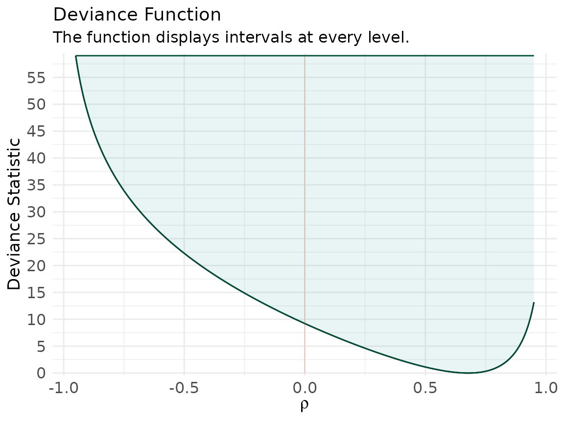
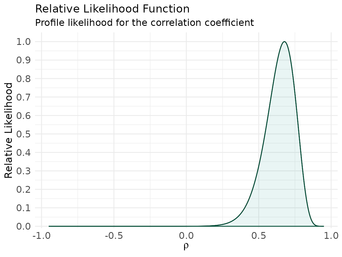
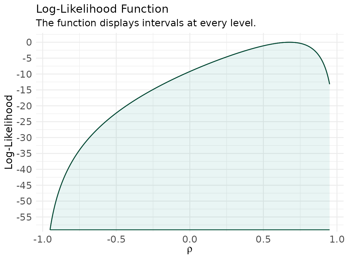
The maximum of the relative likelihood sits at the sample correlation , and the null value receives whatever support the data happen to give it — not a verdict, a height.5
Reading support intervals
A pure-likelihood interval collects every whose relative likelihood exceeds a cutoff .2 Royall’s conventional cutoffs are and ; the cutoff is the likelihood interval that, for an approximately normal likelihood, matches the usual 95% interval (since ).
support_interval <- function(df, k) {
  keep <- df$values[df$support >= 1 / k]
  c(lower = min(keep), upper = max(keep))
}

rbind(
  `1/6.8` = support_interval(lik_rho, 6.8),
  `1/8`   = support_interval(lik_rho, 8),
  `1/32`  = support_interval(lik_rho, 32)
)
#>           lower     upper
#> 1/6.8 0.4329716 0.8262938
#> 1/8   0.4202838 0.8326377
#> 1/32  0.3251252 0.8643573
The companion: consonance and surprisal functions
Now the frequentist view. curve_corr() inverts
cor.test() at every level to produce the consonance
(P-value) function and its surprisal transform.3,6
rho_curve <- curve_corr(
  x = x, y = y,
  alternative = "two.sided",
  method = "pearson"
)
ggcurve(rho_curve[[1]],
  type = "c", nullvalue = TRUE,
  xaxis = expression(rho),
  title = "Consonance (P-value) Function"
)
ggcurve(rho_curve[[1]],
  type = "s", nullvalue = TRUE,
  xaxis = expression(rho),
  title = "Surprisal (S-value) Function"
)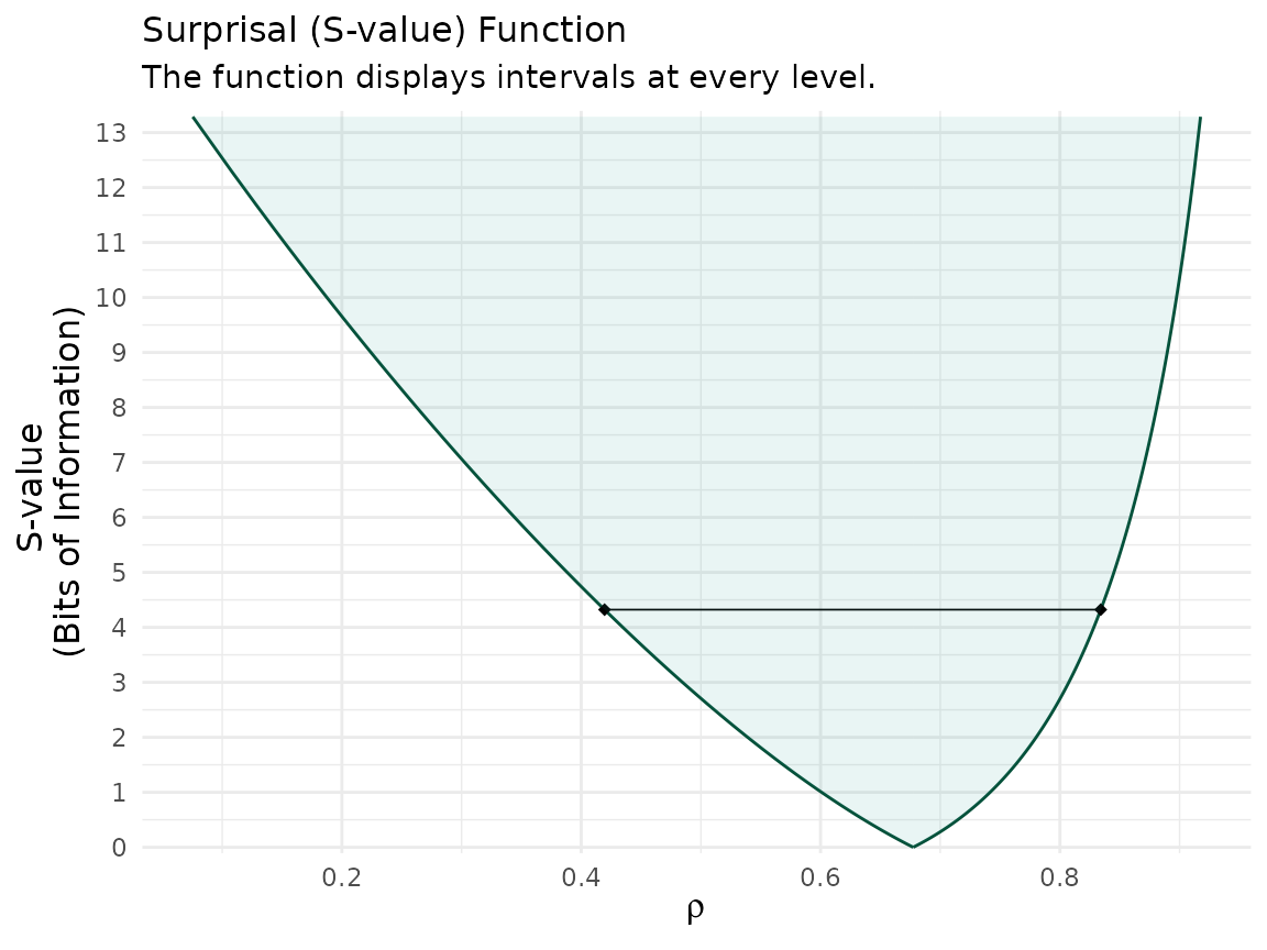
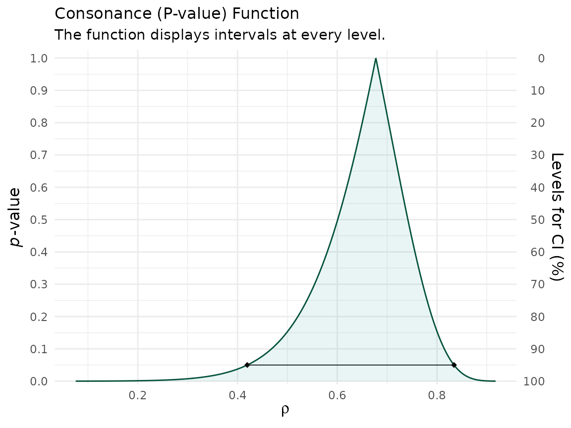
The consonance function peaks at , and its horizontal slice at is the ordinary 95% interval. The surprisal function rescales the same curve into bits of information against each value of .3
The two views agree
The likelihood interval and the 95% consonance interval should land in nearly the same place — that is the whole point.
ci95 <- as.numeric(rho_curve[[1]][
  which.min(abs(rho_curve[[1]]$intrvl.level - 0.95)),
  c("lower.limit", "upper.limit")
])

rbind(
  `Likelihood 1/6.8` = support_interval(lik_rho, 6.8),
  `Consonance 95%`   = c(lower = ci95[1], upper = ci95[2])
)
#>                      lower     upper
#> Likelihood 1/6.8 0.4329716 0.8262938
#> Consonance 95%   0.4195070 0.8341067
They are close but not identical: the likelihood interval is exact
for the profiled normal model, while cor.test() uses
Fisher’s
approximation. The small gap is a feature to notice, not a bug to hide —
it is the difference between two legitimate inferential summaries.1
Cite R Packages
Please remember to cite the packages that you use.
citation("concurve")
#> To cite package 'concurve' in publications use:
#>
#>   Rafi Z, Vigotsky A (2026). _concurve: Computes and Plots
#>   Compatibility (Confidence) Intervals, P-Values, S-Values, &
#>   Likelihood Intervals to Form Consonance, Surprisal, & Likelihood
#>   Functions_. R package version 3.0.5,
#>   <https://CRAN.R-project.org/package=concurve>.
#>
#>   Rafi Z, Greenland S (2020). "Semantic and Cognitive Tools to Aid
#>   Statistical Science: Replace Confidence and Significance by
#>   Compatibility and Surprise." _BMC Medical Research Methodology_,
#>   *20*, 244. ISSN 1471-2288. doi:10.1186/s12874-020-01105-9
#>   <https://doi.org/10.1186/s12874-020-01105-9>.
#>   <https://doi.org/10.1186/s12874-020-01105-9>.
#>
#> To see these entries in BibTeX format, use 'print(<citation>,
#> bibtex=TRUE)', 'toBibtex(.)', or set
#> 'options(citation.bibtex.max=999)'.