Constructing Valid Likelihood Functions • concurve

A likelihood function is only as trustworthy as the model it comes from. It is easy to plot a Gaussian bump centered on an estimate and call it a likelihood; it is harder — and more honest — to write down the exact likelihood a design implies and plot that.¹ This vignette builds several likelihood functions from first principles, each valid for its design, and coerces each into the data-frame layout concurve uses so that ggcurve() can draw it. Where an exact likelihood eliminates a nuisance parameter by conditioning, we use the conditional likelihood rather than a normal approximation.²

Every construction below is checked: its maximum lands on the estimator the design defines. A standalone script, verify-likelihoods.R, repeats those checks as assertions.

A small helper

Each construction produces a vector of parameter values and a relative log-likelihood. This helper normalizes and packages them into the five columns concurve expects (values, likelihood, loglikelihood, support, deviancestat) — the same object curve_lik() returns.

as_concurve_lik <- function(values, loglik) {
  loglik_rel <- loglik - max(loglik)   # relative log-likelihood, max = 0
  support    <- exp(loglik_rel)         # relative likelihood in (0, 1]
  df <- data.frame(
    values        = values,
    likelihood    = support,            # relative likelihood      -> type = "l3"
    loglikelihood = loglik_rel,         # relative log-likelihood   -> type = "l2"
    support       = support,            # relative likelihood       -> type = "l1"
    deviancestat  = -loglik_rel         # -log relative likelihood  -> type = "d"
  )
  class(df) <- c("data.frame", "concurve")
  df
}

# collect every rho whose relative likelihood clears the 1/k cutoff
support_interval <- function(df, k) {
  keep <- df$values[df$support >= 1 / k]
  c(lower = min(keep), upper = max(keep))
}

1. A single proportion: the exact binomial likelihood

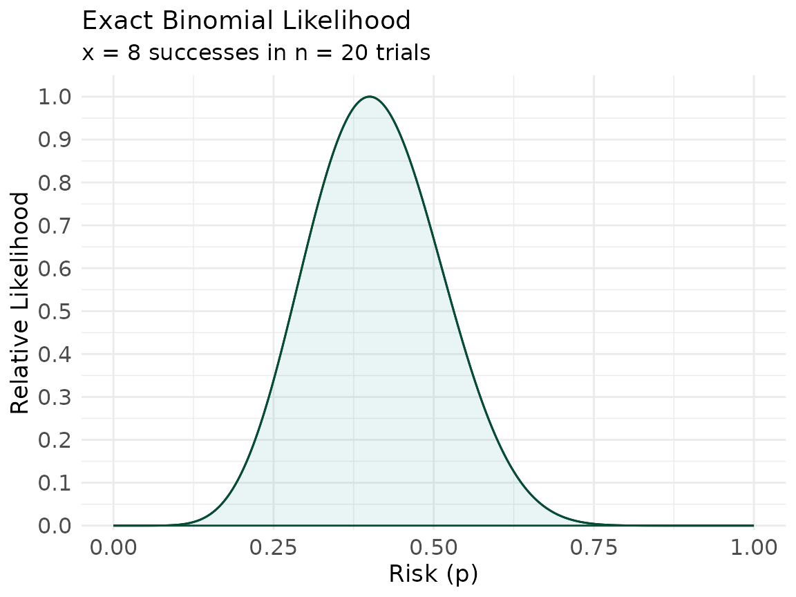
With $x$ successes in $n$ independent trials, the likelihood of the risk $p$ is binomial, $L(p) \propto p^{x}(1-p)^{n-x}$ , and its maximum is the sample proportion $\hat p = x/n$ . No approximation is needed — this is the likelihood.

x <- 8; n <- 20
phat <- x / n

p <- seq(1e-4, 1 - 1e-4, length.out = 4000)
loglik_binom <- x * log(p) + (n - x) * log(1 - p)
lik_p <- as_concurve_lik(p, loglik_binom)

ggcurve(lik_p, type = "l1", nullvalue = TRUE,
        xaxis = "Risk (p)",
        title = "Exact Binomial Likelihood",
        subtitle = sprintf("x = %d successes in n = %d trials", x, n))

Why “exact” earns its keep

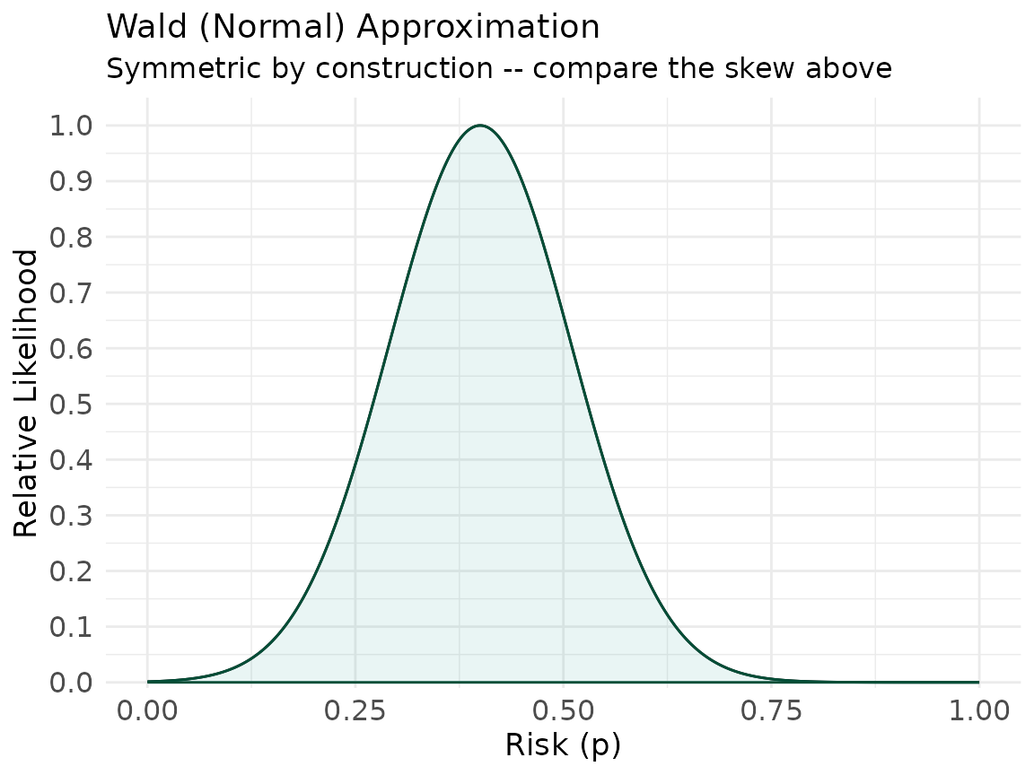
The Wald approximation replaces this with a symmetric Gaussian of variance $\hat p(1-\hat p)/n$ . Near the boundaries the two disagree visibly — the exact likelihood is skewed and respects $0 < p < 1$ , while the Wald bump does not.³

se_wald <- sqrt(phat * (1 - phat) / n)
loglik_wald <- -0.5 * (p - phat)^2 / se_wald^2
lik_p_wald <- as_concurve_lik(p, loglik_wald)

ggcurve(lik_p_wald, type = "l1", nullvalue = TRUE,
        xaxis = "Risk (p)",
        title = "Wald (Normal) Approximation",
        subtitle = "Symmetric by construction -- compare the skew above")

rbind(
  exact = support_interval(lik_p, 6.8),
  wald  = support_interval(lik_p_wald, 6.8)
)
#>           lower     upper
#> exact 0.2073604 0.6166308
#> wald  0.1856093 0.6143807

The exact interval is the one to report; the Wald interval is what happens when you let algebra outrun the data.

2. An odds ratio: the exact conditional likelihood

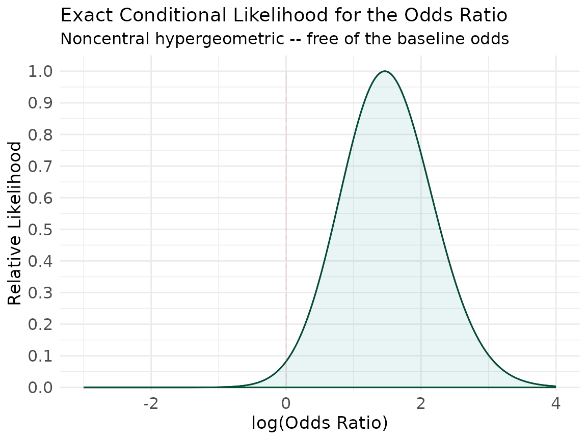
For a $2 \times 2$ table, conditioning on both margins removes the nuisance baseline odds and leaves an exact likelihood for the odds ratio $\psi$ — the noncentral hypergeometric.² If the exposed-case count is $a$ , with exposed total $n_1$ , unexposed total $n_0$ , and case total $m_1$ ,

$\ell(\psi) = a\log\psi \;-\; \log\!\sum_{k}\binom{n_1}{k}\binom{n_0}{m_1-k}\psi^{k},$

summed over the feasible range of $k$ . We plot on the log-OR scale, where the null is $0$ .

# table:            D+   D-
#         E+         a    b
#         E-         c    d
a <- 12; b <- 8; c <- 5; d <- 15
n1 <- a + b; n0 <- c + d; m1 <- a + c

cond_loglik_or <- function(logpsi) {
  klo <- max(0, m1 - n0); khi <- min(m1, n1)
  k <- klo:khi
  logterms <- lchoose(n1, k) + lchoose(n0, m1 - k) + k * logpsi
  M <- max(logterms)
  logZ <- M + log(sum(exp(logterms - M)))   # log-sum-exp for stability
  a * logpsi - logZ
}

logpsi <- seq(-3, 4, length.out = 4000)
loglik_or <- vapply(logpsi, cond_loglik_or, numeric(1))
lik_or <- as_concurve_lik(logpsi, loglik_or)

ggcurve(lik_or, type = "l1", nullvalue = 0,
        xaxis = "log(Odds Ratio)",
        title = "Exact Conditional Likelihood for the Odds Ratio",
        subtitle = "Noncentral hypergeometric -- free of the baseline odds")
#> Warning: Using `size` aesthetic for lines was deprecated in ggplot2 3.4.0.
#> ℹ Please use `linewidth` instead.
#> ℹ The deprecated feature was likely used in the concurve package.
#>   Please report the issue at <https://github.com/zadrafi/concurve/issues>.
#> This warning is displayed once per session.
#> Call `lifecycle::last_lifecycle_warnings()` to see where this warning was
#> generated.


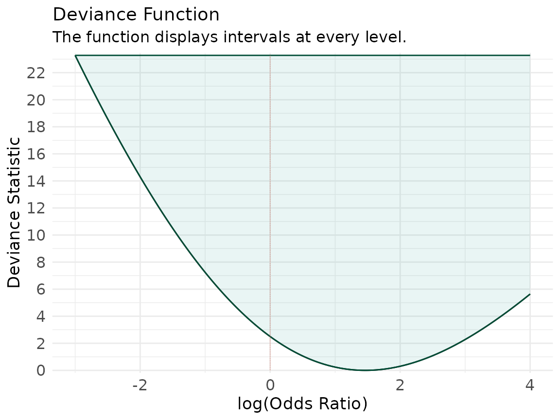
ggcurve(lik_or, type = "d", nullvalue = 0,
        xaxis = "log(Odds Ratio)",
        title = "Deviance Function")

Note the peak: the conditional likelihood is maximized at the conditional MLE, which is close to but not identical to the naive cross-product $ad/bc$ .

c(
  `sample ad/bc`   = (a * d) / (b * c),
  `conditional MLE`= exp(lik_or$values[which.max(lik_or$support)])
)
#>    sample ad/bc conditional MLE 
#>        4.500000        4.321558

That gap is not rounding error — it is the difference between a marginal summary and the estimator the exact conditional model actually supports.²

3. A rate ratio: the exact conditional binomial likelihood

Two Poisson counts, $a$ events in person-time $T_1$ and $b$ events in $T_0$ , carry an exact likelihood for the rate ratio $\theta = \lambda_1/\lambda_0$ once you condition on the total number of events. Conditionally, $a \mid (a+b) \sim \text{Binomial}(a+b,\ \pi)$ with $\pi(\theta) = \theta T_1 / (\theta T_1 + T_0)$ .⁴

a_e <- 30; T1 <- 1000   # exposed:   events, person-time
b_e <- 18; T0 <- 1200   # unexposed: events, person-time

cond_loglik_rr <- function(logtheta) {
  theta <- exp(logtheta)
  pi <- theta * T1 / (theta * T1 + T0)
  a_e * log(pi) + b_e * log(1 - pi)
}

logtheta <- seq(-2, 3, length.out = 4000)
loglik_rr <- vapply(logtheta, cond_loglik_rr, numeric(1))
lik_rr <- as_concurve_lik(logtheta, loglik_rr)

ggcurve(lik_rr, type = "l1", nullvalue = 0,
        xaxis = "log(Rate Ratio)",
        title = "Exact Conditional Likelihood for the Rate Ratio",
        subtitle = "Binomial conditional on total events -- no offset approximation")

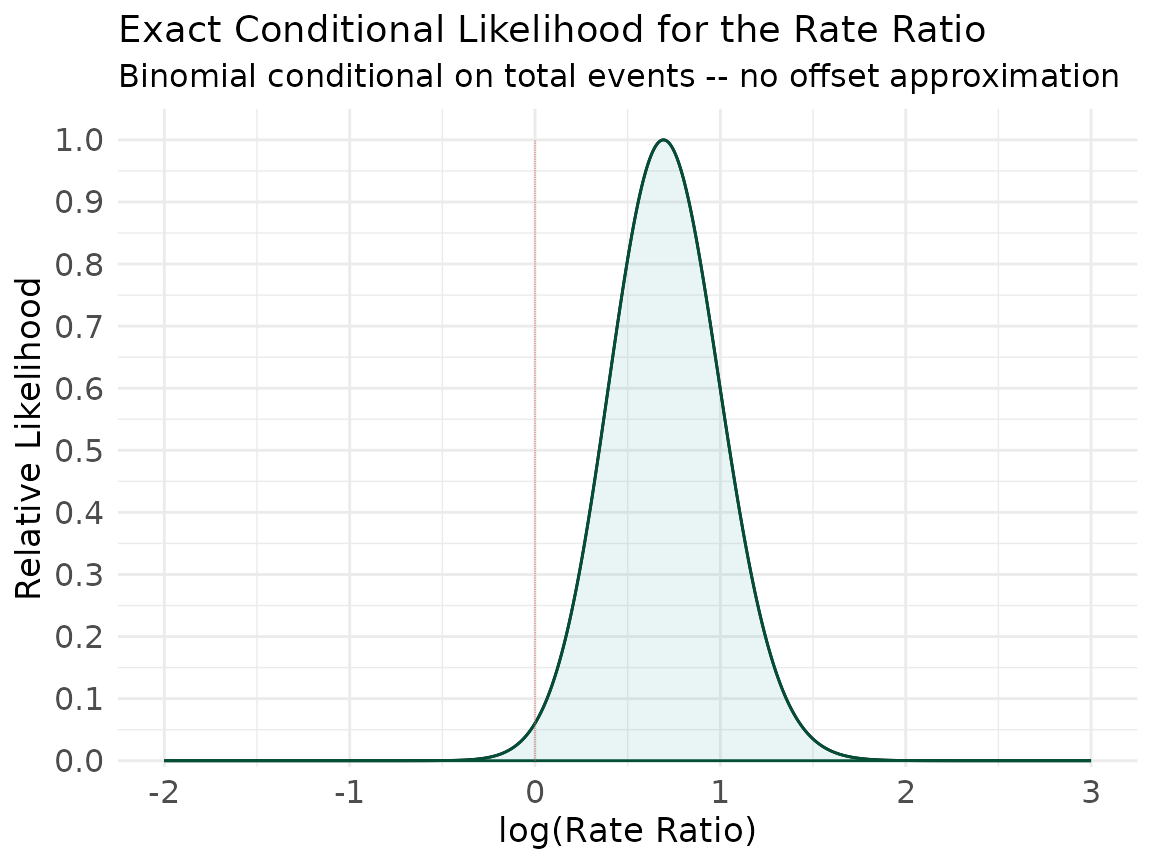
Here the conditional MLE is the sample rate ratio exactly:

c(
  `sample RR`      = (a_e / T1) / (b_e / T0),
  `likelihood peak`= exp(lik_rr$values[which.max(lik_rr$support)])
)
#>       sample RR likelihood peak 
#>        2.000000        2.000052

4. A mean: the profile likelihood

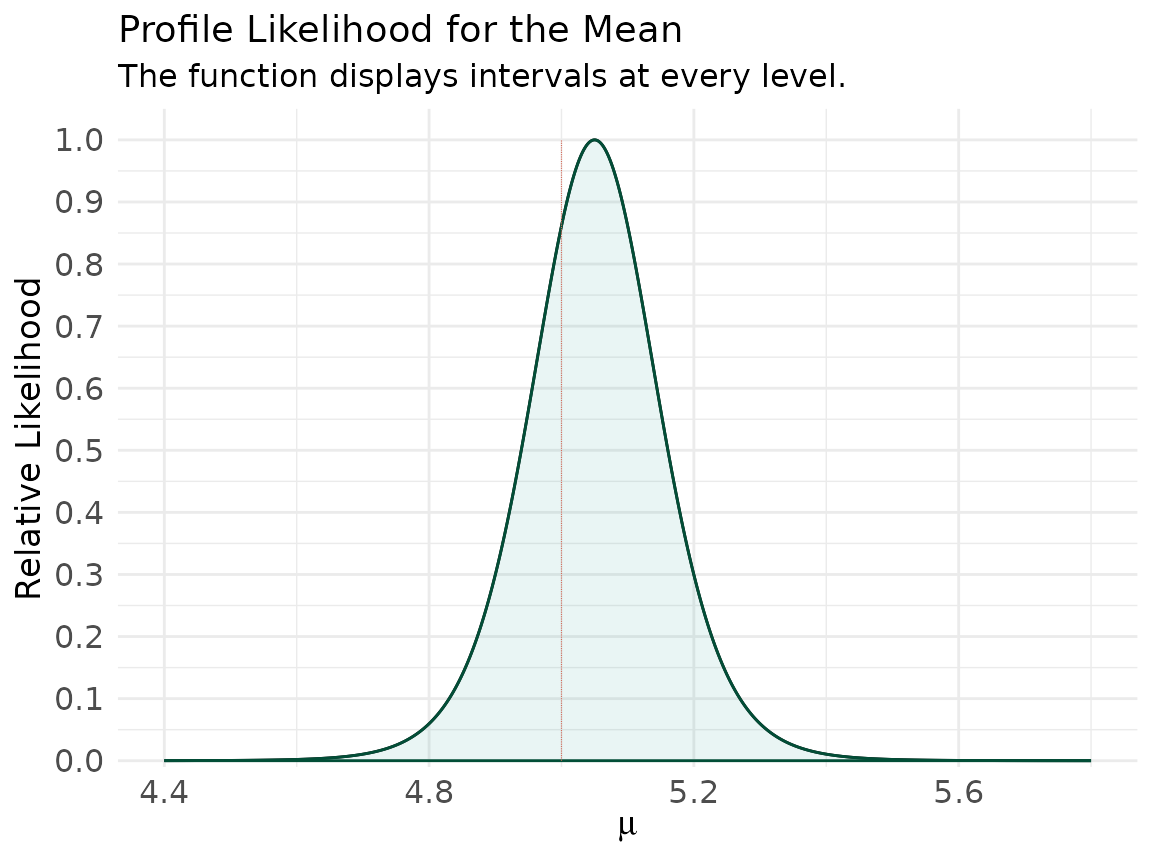
For a normal sample, profiling out the unknown variance leaves a profile likelihood for the mean $\mu$ that depends only on the residual sum of squares (Pawitan, In All Likelihood, 2001):¹

$\ell_p(\mu) = -\frac{n}{2}\log\!\left(\frac{\sum_i (x_i - \mu)^2}{\sum_i (x_i - \bar x)^2}\right).$

xs <- c(5.1, 4.8, 5.5, 4.9, 5.3, 5.0, 4.7, 5.2, 5.4, 4.6)
n_x <- length(xs); xbar <- mean(xs)
ss_min <- sum((xs - xbar)^2)

mu <- seq(4.4, 5.8, length.out = 4000)
loglik_mu <- -(n_x / 2) * log(vapply(mu, function(m) sum((xs - m)^2), numeric(1)) / ss_min)
lik_mu <- as_concurve_lik(mu, loglik_mu)

ggcurve(lik_mu, type = "l1", nullvalue = 5.0,
        xaxis = expression(mu),
        title = "Profile Likelihood for the Mean")

5. A variance (and SD): the chi-square likelihood

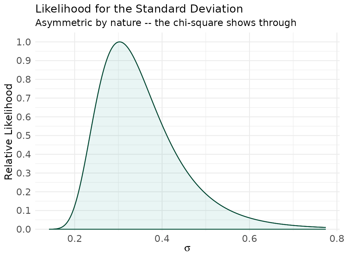
The likelihood for a variance $\sigma^2$ follows from the sampling distribution of $s^2$ , since $\nu s^2 / \sigma^2 \sim \chi^2_\nu$ with $\nu = n-1$ . It is genuinely asymmetric — a shape people rarely see plotted because the Wald habit hides it. We plot it on the standard- deviation scale by mapping $\sigma = \sqrt{\sigma^2}$ .

s2 <- var(xs); nu <- n_x - 1

sig2 <- seq(0.02, 0.60, length.out = 4000)
loglik_var <- -(nu / 2) * log(sig2) - nu * s2 / (2 * sig2)
lik_sd <- as_concurve_lik(sqrt(sig2), loglik_var)   # values on the SD scale

ggcurve(lik_sd, type = "l1", nullvalue = TRUE,
        xaxis = expression(sigma),
        title = "Likelihood for the Standard Deviation",
        subtitle = "Asymmetric by nature -- the chi-square shows through")

What made each of these valid

None of these leaned on a Gaussian approximation to the log-likelihood. The proportion used the binomial directly; the odds ratio and rate ratio used exact conditional likelihoods that delete their nuisance parameters by conditioning on sufficient margins; the mean and variance came from the exact normal-theory sampling distributions.^1,2 Each maximum coincides with the estimator its design defines (the odds-ratio conditional MLE included), and each function is skewed exactly as much as the model says it should be — which is the information a single interval throws away.^5,6

Once an object is in concurve form, everything else in the package — support intervals, deviance and log-likelihood views, side-by-side comparison with a consonance function — works on it unchanged.

Cite R Packages

Please remember to cite the packages that you use.

citation("concurve")
#> To cite package 'concurve' in publications use:
#> 
#>   Rafi Z, Vigotsky A (2026). _concurve: Computes and Plots
#>   Compatibility (Confidence) Intervals, P-Values, S-Values, &
#>   Likelihood Intervals to Form Consonance, Surprisal, & Likelihood
#>   Functions_. R package version 3.0.0,
#>   <https://CRAN.R-project.org/package=concurve>.
#> 
#>   Rafi Z, Greenland S (2020). "Semantic and Cognitive Tools to Aid
#>   Statistical Science: Replace Confidence and Significance by
#>   Compatibility and Surprise." _BMC Medical Research Methodology_,
#>   *20*, 244. ISSN 1471-2288. doi:10.1186/s12874-020-01105-9
#>   <https://doi.org/10.1186/s12874-020-01105-9>.
#>   <https://doi.org/10.1186/s12874-020-01105-9>.
#> 
#> To see these entries in BibTeX format, use 'print(<citation>,
#> bibtex=TRUE)', 'toBibtex(.)', or set
#> 'options(citation.bibtex.max=999)'.

References

Royall R. Statistical Evidence: A Likelihood Paradigm. CRC Press; 1997.

Cox DR, Hinkley DV. Theoretical Statistics. Chapman and Hall/CRC; 1974. doi:10.1201/b14832

Rothman KJ, Greenland S, Lash TL. Modern Epidemiology. 3rd ed. Lippincott Williams & Wilkins; 2008. https://books.google.com/books/about/Modern_Epidemiology.html?id=Z3vjT9ALxHUC.

Cummings P. Analysis of Incidence Rates. CRC Press; 2019. https://doi.org/10.1201/9780429055713.

Rafi Z, Greenland S. Semantic and cognitive tools to aid statistical science: Replace confidence and significance by compatibility and surprise. BMC Medical Research Methodology. 2020;20(1):244. doi:10.1186/s12874-020-01105-9

Poole C. Confidence intervals exclude nothing. American Journal of Public Health. 1987;77(4):492-493. doi:10.2105/ajph.77.4.492