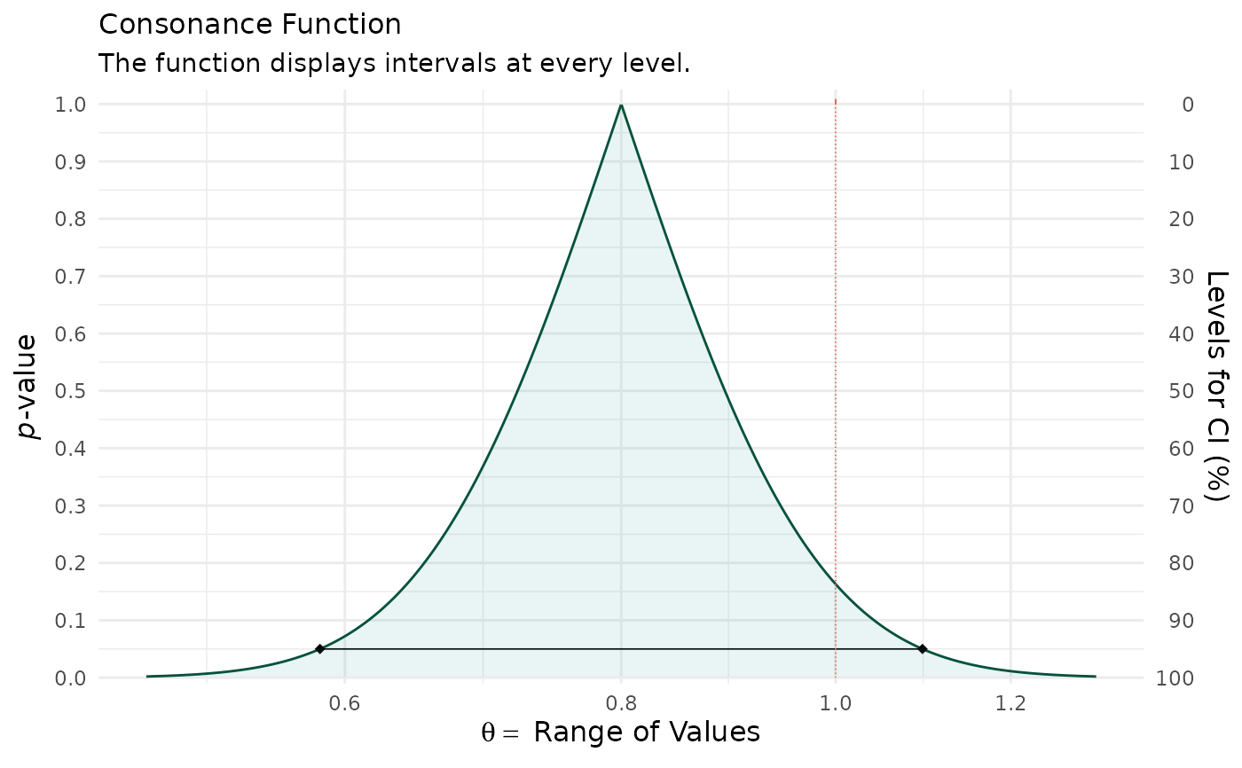
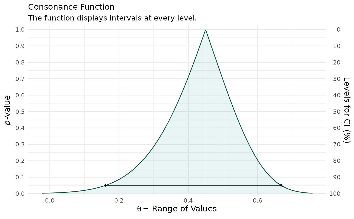
Analytic Consonance Functions From Summary Statistics

Computes consonance (confidence) intervals at every level directly from closed-form quantile functions rather than by numerically inverting confint() thousands of times. This is exact for the stated sampling model, requires no fitted model object, produces no profiling messages, and is typically several orders of magnitude faster than the inversion-based functions. The output object is identical in structure to that of curve_gen(), so ggcurve(), curve_compare(), plot_compare(), and curve_table() all work on it unchanged.

curve_analytic(estimate, se = NULL, df = NULL, n = NULL, dist = c("z",
  "t", "corr", "var", "prop"), log = FALSE, penalty = NULL, m = NULL,
  steps = 1000, table = TRUE)

Arguments

estimate

The point estimate. For dist = "corr" this is the sample correlation coefficient; for dist = "var" the sample variance; for dist = "prop" the number of successes (a count, together with n).

se

The standard error of the estimate. Required for dist = "z" and dist = "t". Ignored otherwise.

df

Degrees of freedom. Required for dist = "t".

n

The sample size. Required for dist = "corr", dist = "var", and dist = "prop".

dist

The sampling distribution used to construct the intervals:

"z": Normal (Wald) intervals, estimate and se.
"t": Student-t intervals, estimate, se, and df.
"corr": Pearson correlation via the Fisher z-transformation, estimate (r) and n; the standard error on the z scale is 1/sqrt(n - 3).
"var": A normal-model variance via the chi-squared pivot (n - 1) s^2 / sigma^2, estimate (s^2) and n.
"prop": A binomial proportion via the Wilson score interval, estimate (number of successes) and n.

log

Indicates whether the estimate is on the log scale and the limits should be exponentiated (as when supplying a log risk ratio, log odds ratio, or log hazard ratio with its standard error). Defaults to FALSE. Only available for dist = "z" and dist = "t".

penalty

An input to specify whether the intervals should be corrected for multiple comparisons. The default is NULL, so there is no correction. Other options include "bonferroni" and "sidak".

m

Indicates how many comparisons are being done and the number that should be used to correct for multiple comparisons. The default is NULL.

steps

Indicates how many consonance intervals are to be calculated at various levels. By default, it is set to 1000. Because the limits are computed analytically, large values are cheap.

table

Indicates whether or not a table output with some relevant statistics should be generated. The default is TRUE and generates a table which is included in the list object.

Value

A list with 3 items where the dataframe of values is in the first object, the values needed to calculate the density function in the second, and the table for the values in the third if table = TRUE.

Details

The analytic approach follows the confidence-distribution framework reviewed by Xie & Singh (2013) and implemented for several estimate types by Infanger & Schmidt-Trucksäss (2019) in the pvaluefunctions package: for each interval level the limits are read off the quantile function of the estimator's sampling distribution.

References

Xie M, Singh K. Confidence distribution, the frequentist distribution estimator of a parameter: a review. Int Stat Rev. 2013;81(1):3-39.

Infanger D, Schmidt-Trucksäss A. P value functions: An underused method to present research results and to promote quantitative reasoning. Stat Med. 2019;38(21):4189-4197.

Rafi Z, Greenland S. Semantic and cognitive tools to aid statistical science: replace confidence and significance by compatibility and surprise. BMC Med Res Methodol. 2020;20(1):244.

Examples

# From a log hazard ratio and its SE, on the ratio scale:
hr <- curve_analytic(estimate = log(0.80), se = 0.16, dist = "z", log = TRUE)
ggcurve(hr[[1]], measure = "ratio", nullvalue = 1)
#> Warning: Using `size` aesthetic for lines was deprecated in ggplot2 3.4.0.
#> ℹ Please use `linewidth` instead.
#> ℹ The deprecated feature was likely used in the concurve package.
#>   Please report the issue at <https://github.com/zadrafi/concurve/issues>.


# A correlation from r and n:
rho <- curve_analytic(estimate = 0.45, n = 40, dist = "corr")
ggcurve(rho[[1]])